Light Curve Classifier

Learning Goals

By the end of this tutorial, you will be able to:

• prepare data for ML algorithms by cleaning and filtering the dataset

• work with Pandas dataframes as a way of storing and manipulating time domain datasets

• use sktime algorithms to train a classifier and calculate metrics of accuracy

• use the trained classifier to predict labels on an unlabelled dataset

Introduction

The science goal of this notebook is to find a classifier that can accurately discern changing look active galactic nuclei (CLAGN) from a broad sample of all Sloan Digital Sky Survey (SDSS) identified Quasars (QSOs) based solely on archival photometry in the form of multiwavelength light curves.

CLAGN are astrophysically interesting objects because they appear to change state. CLAGN are characterized by the appearance or disappearance of broad emission lines on timescales of order months. Astronomers would like to understand the physical mechanism behind this apparent change of state. However, only a few hundered CLAGN are known, and finding CLAGN is observationally expensive, traditionally requiring multiple epochs of spectroscopy. Being able to identify CLAGN in existing, archival, large, photometric samples would allow us to identify a statisitcally significant sample from which we could better understand the underlying physics.

This notebook walks through an exercise in using multiwavelength photometry(no spectroscopy) to learn if we can identify CLAGN based on their light curves alone. If we are able to find a classifier that can differentiate CLAGN from SDSS QSOs, we would then be able to run the entire sample of SDSS QSOs (~500,000) to find additional CLAGN candidates for follow-up verification.

Input to this notebook is output of a previous demo notebook which generates multiwavelength light curves from archival data. This notebook starts with light curves, does data prep, and runs the light curves through multiple ML classification algorithms. There are many ML algorthms to choose from; We choose to use sktime algorithms for time domain classification beacuse it is a library of many algorithms specifically tailored to time series datasets. It is based on the scikit-learn library so syntax is familiar to many users.

The challenges of this time-domain dataset for ML work are:

1. Multi-variate = There are multiple bands of observations per target (13+)

2. Unequal length = Each band has a light curve with different sampling than other bands

3. Missing data = Not each object has all observations in all bands

Input

Light curve parquet file of multiwavelength light curves from the light_curve_generator.md demo notebook in this same repo. The format of the light curves is a Pandas multiindex data frame.

We choose to use a Pandas multiindex dataframe to store and work with the data because it fulfills these requirements:

1. It can handle the above challenges of a dataset = multi-variate, unqueal length with missing data.

2. Multiple targets (multiple rows)

3. Pandas has some built in understanding of time units

4. Can be scaled up to big data numbers of rows (altough we don’t push to out of memory structures in this use case)

5. Pandas is user friendly with a lot of existing functionality

A useful reference for what sktime expects as input to its ML algorithms: https://github.com/sktime/sktime/blob/main/examples/AA_datatypes_and_datasets.ipynb

Output

Trained classifiers as well as estimates of their accuracy and plots of confusion matrices

Runtime

As of 2024 August, this notebook takes ~170s to run to completion on Fornax using the ‘Astrophysics Default Image’ and the ‘Large’ server with 16GB RAM/ 4CPU.

Authors

Jessica Krick, Shoubaneh Hemmati, Troy Raen, Brigitta Sipőcz, Andreas Faisst, Vandana Desai, David Shupe

Acknowledgements

Stephanie La Massa

Imports

• pandas to work with light curve data structure

• numpy for numerical calculations

• matplotlib for plotting

• sys for paths

• astropy to work with coordinates/units and data structures

• tqdm for showing progress meter

• sktime ML algorithms specifically for time-domain data

• sklearn general use ML algorthims with easy to use interface

• scipy for statistical analysis

• json for storing intermediate files

• google_drive_downloader to access files stored in google drive

This cell will install them if needed:

# Uncomment the next line to install dependencies if needed.
# !pip install -r requirements_light_curve_classifier.txt

import sys

import matplotlib.pyplot as plt
from matplotlib.lines import Line2D
import pandas as pd
from astropy.table import Table
from google_drive_downloader import GoogleDriveDownloader as gdd
from tqdm.auto import tqdm
import json

from sklearn.metrics import ConfusionMatrixDisplay, accuracy_score, confusion_matrix
from sklearn.model_selection import train_test_split
from sklearn.gaussian_process import GaussianProcessRegressor
from sklearn.gaussian_process.kernels import RBF

from sktime.classification.deep_learning import CNNClassifier
from sktime.classification.dictionary_based import IndividualTDE
from sktime.classification.distance_based import KNeighborsTimeSeriesClassifier
from sktime.classification.dummy import DummyClassifier
from sktime.classification.ensemble import WeightedEnsembleClassifier
from sktime.classification.feature_based import Catch22Classifier, RandomIntervalClassifier
from sktime.classification.hybrid import HIVECOTEV2
from sktime.classification.interval_based import CanonicalIntervalForest
from sktime.classification.kernel_based import Arsenal, RocketClassifier
from sktime.classification.shapelet_based import ShapeletTransformClassifier
from sktime.registry import all_estimators, all_tags
from sktime.datatypes import check_is_mtype

# local code imports
sys.path.append('code_src/')
from classifier_functions import sigmaclip_lightcurves, remove_objects_without_band, \
remove_incomplete_data, missingdata_to_zeros, missingdata_drop_bands, \
uniform_length_spacing, reformat_df, local_normalization_max, mjd_to_datetime

#improves memory usage and avoids problems that trigger warnings
pd.options.mode.copy_on_write = True

1. Read in a dataset of archival light curves

We use here a sample of AGN including known CLAGN & random SDSS AGN

If you want to use your own sample, you can use the code light_curve_generator.md in this same repo to make the required pandas dataframe which you will need to run this notebook.

# First we want to load light curves made in the light curve generator notebook

# The data is on google drive, this will download it for you and read it into
# a pandas dataframe
savename_df_lc = './data/small_CLAGN_SDSS_df_lc.parquet'
gdd.download_file_from_google_drive(file_id='1DrB-CWdBBBYuO0WzNnMl5uQnnckL7MWH',
                                    dest_path=savename_df_lc,
                                    unzip=True)

#load the data into a pandas dataframe
df_lc = pd.read_parquet(savename_df_lc)

Downloading 1DrB-CWdBBBYuO0WzNnMl5uQnnckL7MWH into ./data/small_CLAGN_SDSS_df_lc.parquet... 

Done.
Unzipping...

/home/runner/work/fornax-demo-notebooks/fornax-demo-notebooks/.tox/py311-buildhtml/lib/python3.11/site-packages/google_drive_downloader/google_drive_downloader.py:78: UserWarning: Ignoring `unzip` since "1DrB-CWdBBBYuO0WzNnMl5uQnnckL7MWH" does not look like a valid zip file
  warnings.warn('Ignoring `unzip` since "{}" does not look like a valid zip file'.format(file_id))

#get rid of indices set in the light curve code and reset them as needed
#before sktime algorithms
df_lc = df_lc.reset_index()

#what does the dataset look like at the start?
df_lc

	objectid	label	band	time	flux	err
0	15	MacLeod 19	SAXGRBMGRB	50335.861597	0.100000	0.1
1	240	SDSS	SAXGRBMGRB	51601.900023	0.100000	0.1
2	364	SDSS	SAXGRBMGRB	50594.078796	0.100000	0.1
3	169	SDSS	SAXGRBMGRB	51373.759595	0.100000	0.1
4	446	SDSS	SAXGRBMGRB	50991.525394	0.100000	0.1
...	...	...	...	...	...	...
458312	453	SDSS	K2	60148.521180	1.020081	NaN
458313	453	SDSS	K2	60149.195427	1.014221	NaN
458314	453	SDSS	K2	60149.930970	1.009093	NaN
458315	453	SDSS	K2	60150.584787	1.003534	NaN
458316	453	SDSS	K2	60151.238603	1.000992	NaN

458317 rows × 6 columns

2. Data Prep

The majority of work in all ML projects is preparing and cleaning the data. As most do, this dataset needs significant work before it can be fed into a ML algorithm. Data preparation includes everything from removing statistical outliers to putting it in the correct data format for the algorithms.

2.1 Remove bands with not enough data

For this use case of CLAGN classification, we don’t need to include some of the bands that are known to be sparse. Most ML algorithms cannot handle sparse data so one way to accomodate that is to remove the sparsest datasets.

##what are the unique set of bands included in our light curves
df_lc.band.unique()

#get rid of some of the bands that don't have enough data for all the sources
#CLAGN are generall fainter targets, and therefore mostly not found
#in datasets like TESS & K2

bands_to_drop = ["IceCube", "TESS", "FERMIGTRIG", "K2"]
df_lc = df_lc[~df_lc["band"].isin(bands_to_drop)]

2.2 Combine Labels for a Simpler Classification

All CLAGN start in the dataset as having labels based on their discovery paper. Because we want one sample with all known CLAGN, we change those discovery names to be simply “CLAGN” for all CLAGN, regardless of origin.

df_lc['label'] = df_lc.label.str.replace('MacLeod 16', 'CLAGN')
df_lc['label'] = df_lc.label.str.replace('LaMassa 15', 'CLAGN')
df_lc['label'] = df_lc.label.str.replace('Yang 18', 'CLAGN')
df_lc['label'] = df_lc.label.str.replace('Lyu 22', 'CLAGN')
df_lc['label'] = df_lc.label.str.replace('Hon 22', 'CLAGN')
df_lc['label'] = df_lc.label.str.replace('Sheng 20', 'CLAGN')
df_lc['label'] = df_lc.label.str.replace('MacLeod 19', 'CLAGN')
df_lc['label'] = df_lc.label.str.replace('Green 22', 'CLAGN')
df_lc['label'] = df_lc.label.str.replace('Lopez-Navas 22', 'CLAGN')

print(df_lc.groupby(["objectid"]).ngroups, "n objects before removing missing band data")

451 n objects before removing missing band data

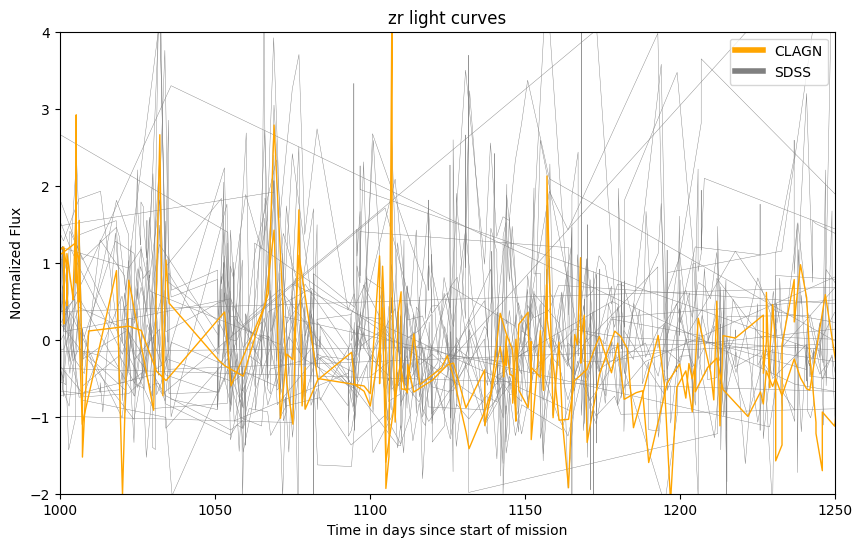
2.3 Data Visualization

• can we see any trends by examining plots of a subset of the data?

#chhose your own adventure, the bands from which you can choose are:
df_lc.band.unique()

array(['SAXGRBMGRB', 'G', 'BP', 'RP', 'panstarrs i', 'panstarrs y',
       'panstarrs z', 'panstarrs g', 'panstarrs r', 'zg', 'zi', 'zr',
       'W1', 'W2', 'k2'], dtype=object)

#plot a single band for all objects
band_of_interest = 'zr'
band_lc = df_lc[df_lc['band'] == band_of_interest]
#reset zero time to be start of that mission
band_lc["time"] = band_lc["time"] - band_lc["time"].min()
band_lc.time.min()

band_lc.set_index('time', inplace = True)  #helps with the plotting

#drop some objects to try to clear up plot
querystring1 = 'objectid < 162'
querystring2 = 'objectid > 200'
band_lc = band_lc.drop(band_lc.query(querystring1 ).index)
band_lc = band_lc.drop(band_lc.query(querystring2 ).index)

#quick normalization for plotting
#we normalize for real after cleaning the data
# make a new column with max_r_flux for each objectid
band_lc['mean_band'] = band_lc.groupby('objectid', sort=False)["flux"].transform('mean')
band_lc['sigma_band'] = band_lc.groupby('objectid', sort=False)["flux"].transform('std')

#choose to normalize (flux - mean) / sigma
band_lc['flux'] = (band_lc['flux'] - band_lc['mean_band']).div(band_lc['sigma_band'], axis=0)

#want to have two different sets so I can color code
clagn_df = band_lc[band_lc['label'] == 'CLAGN']
sdss_df = band_lc[band_lc['label'] == 'SDSS']
print(clagn_df.groupby(["objectid"]).ngroups, "n objects CLAGN ")
print(sdss_df.groupby(["objectid"]).ngroups, "n objects SDSS ")

#groupy objectid & plot flux vs. time
fig, ax = plt.subplots(figsize=(10,6))
lc_sdss = sdss_df.groupby(['objectid'])['flux'].plot(kind='line', ax=ax, color = 'gray', label = 'SDSS', linewidth = 0.3)
lc_clagn = clagn_df.groupby(['objectid'])['flux'].plot(kind='line', ax=ax, color = 'orange', label = 'CLAGN', linewidth = 1)

#add legend and labels/titles
legend_elements = [Line2D([0], [0], color='orange', lw=4, label='CLAGN'),
                   Line2D([0], [0], color='gray', lw=4, label='SDSS')]
ax.legend(handles=legend_elements, loc='best')

ax.set_ylabel('Normalized Flux')
ax.set_xlabel('Time in days since start of mission')
plt.title(f"{band_of_interest} light curves")

#tailored to ZTF r band with lots of data
ax.set_ylim([-2, 4])
ax.set_xlim([1000, 1250])

2 n objects CLAGN 
34 n objects SDSS 

(1000.0, 1250.0)

2.4 Clean the dataset of unwanted data

“unwanted” includes:

• NaNs

  • SKtime does not work with NaNs

• zero flux

  • there are a few flux measurements that come into our dataframe with zeros. It is not clear what these are, and zero will be used to mean lack of observation in the rest of this notebook, so want to drop these rows at the outset.

• outliers in uncertainty

  • This is a tricky job because we want to keep astrophysical sources that are variable objects, but remove instrumental noise and CR (ground based). The user will need to choose a sigma clipping threshold, and there is some plotting functionality available to help users make that decision

• objects with no measurements in WISE W1 band

  • Below we want to normalize all light curves by W1, so we neeed to remove those objects without W1 fluxes because there will be nothing to normalize those light curves with. We don’t want to have un-normalized data.

• objects with incomplete data

  • Incomplete is defined here as not enough flux measurements to make a good light curve. Some bands in some objects have only a few datapoints. Three data points is not large enough for KNN interpolation, so we will consider any array with fewer than 4 photometry points to be incomplete data. Another way of saying this is that we choose to remove those light curves with 3 or fewer data points.

#drop rows which have Nans
df_lc.dropna(inplace = True, axis = 0)

#drop rows with zero flux
querystring = 'flux < 0.000001'
df_lc = df_lc.drop(df_lc.query(querystring).index)

#remove outliers
sigmaclip_value = 10.0
df_lc = sigmaclip_lightcurves(df_lc, sigmaclip_value, include_plot = False)
print(df_lc.groupby(["objectid"]).ngroups, "n objects after sigma clipping")

#remove incomplete data
threshold_too_few = 3
df_lc = remove_incomplete_data(df_lc, threshold_too_few, verbose = False)

#remove objects without W1 fluxes
df_lc = remove_objects_without_band(df_lc, 'W1', verbose=True)

print(df_lc.groupby(["objectid"]).ngroups, "n objects after cleaning the data")

451 n objects after sigma clipping

18 objects without W1  were removed
431 n objects after cleaning the data

2.5 Missing Data

Some objects do not have light curves in all bands. Some ML algorithms can handle mising data, but not all, so we try to do something intentional and sensible to handle this missing data up front.

There are two options here:

1. We will add light curves with zero flux and err values for the missing data. SKtime does not like NaNs, so we choose zeros. This option has the benefit of including more bands and therefore more information, but the drawback of having some objects have bands with entire arrays of zeros.

2. Remove bands which have less data from all objects so that there are no objects with missing data. This has the benefit of less zeros, but the disadvantage of throwing away some information for the few objects which do have light curves in the bands which will be removed.

Functions are inlcuded for both options.

#choose what to do with missing data...
#df_lc = missingdata_to_zeros(df_lc)
#or
bands_to_keep = ['W1','W2','panstarrs g','panstarrs i', 'panstarrs r','panstarrs y','panstarrs z','zg','zr']
df_lc = missingdata_drop_bands(df_lc, bands_to_keep, verbose = True)

431 n objects before removing missing band data
357 n objects after removing missing band data

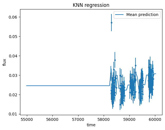
2.6 Make all objects and bands have identical time arrays (uniform length and spacing)

It is very hard to find time-domain ML algorithms which can work with non uniform length datasets. Therefore we make the light curves uniform by interpolating using KNN from scikit-learn which fills in the uniform length arrays with a final frequency chosen by the user. We choose KNN as very straightforward method. This function also shows the framework in case the user wants to choose a different scikit-learn function to do the interpolation. Another natural choice would be to use gaussian processes (GP) to do the interpolation, but this is not a good solution for our task because the flux values go to zero at times before and after the observations. Because we include the entire time array from beginning of the first mission to end of the last mission, most individual bands require interpolation before and after their particular observations. In other words, our light curves span the entire range from 2010 with the start of panstarrs and WISE to the most recent ZTF data release (at least 2023), even though most individual missions do not cover that full range of time.

It is important to choose the frequency over which the data is interpolated wisely. Experimentation with treating this variable like a hyperparam and testing sktime algorithms shows slightly higher accuracy values for a suite of algorithms for a frequency of one interpolated observation per 60 days.

#what does the dataframe look like at this point in the code?
df_lc

	objectid	label	band	time	flux	err
12489	1	CLAGN	panstarrs i	55174.305492	0.100490	0.001102
12490	1	CLAGN	panstarrs i	55174.308519	0.090206	0.000985
12491	1	CLAGN	panstarrs y	55416.614225	0.130497	0.007047
12492	1	CLAGN	panstarrs y	55416.625133	0.133000	0.006277
12493	1	CLAGN	panstarrs z	55427.627576	0.118545	0.002673
...	...	...	...	...	...	...
412825	458	SDSS	W2	58283.310746	1.793368	0.015925
412826	458	SDSS	W2	58490.115697	1.630802	0.017747
412827	458	SDSS	W2	58650.370860	1.674718	0.017944
412828	458	SDSS	W2	58854.359409	1.475255	0.017491
412829	458	SDSS	W2	59014.562406	1.400782	0.017341

346191 rows × 6 columns

#this cell takes 13seconds to run on the sample of 458 sources
#change this to change the frequency of the time array
final_freq_interpol = 60  #this is the timescale of interpolation in units of days

#make all light curves have the same time array
df_interpol = uniform_length_spacing(df_lc, final_freq_interpol, include_plot = True )

# df_lc_interpol has one row per dict in lc_interpol. time and flux columns store arrays.
# "explode" the dataframe to get one row per light curve point. time and flux columns will now store floats.
df_lc = df_interpol.explode(["time", "flux","err"], ignore_index=True)
df_lc = df_lc.astype({col: "float" for col in ["time", "flux", "err"]})

2.7 Restructure dataframe

• Make columns have band names in them and then remove band from the index

• pivot the dataframe so that SKTIME understands its format

• this will put it in the format expected by sktime

#reformat the data to have columns be the different flux bands
df_lc = reformat_df(df_lc)

#look at a single object to see what this array looks like
ob_of_interest = 12
singleob = df_lc[df_lc['objectid'] == ob_of_interest]
singleob

	objectid	label	time	flux_W1	flux_W2	flux_panstarrs_g	flux_panstarrs_i	flux_panstarrs_r	flux_panstarrs_y	flux_panstarrs_z	...	flux_zr	err_W1	err_W2	err_panstarrs_g	err_panstarrs_i	err_panstarrs_r	err_panstarrs_y	err_panstarrs_z	err_zg	err_zr
850	12	CLAGN	54985.275796	0.171426	0.183990	0.014124	0.083940	0.043920	0.068864	0.085598	...	0.065361	0.007365	0.018009	0.00128	0.002069	0.002013	0.007337	0.004	0.003695	0.00521
851	12	CLAGN	55045.275796	0.171426	0.183990	0.014124	0.083940	0.043920	0.068864	0.085598	...	0.065361	0.007365	0.018009	0.00128	0.002069	0.002013	0.007337	0.004	0.003695	0.00521
852	12	CLAGN	55105.275796	0.171426	0.183990	0.014124	0.083940	0.043920	0.068864	0.085598	...	0.065361	0.007365	0.018009	0.00128	0.002069	0.002013	0.007337	0.004	0.003695	0.00521
853	12	CLAGN	55165.275796	0.171426	0.183990	0.014124	0.083940	0.043920	0.068864	0.085598	...	0.065361	0.007365	0.018009	0.00128	0.002069	0.002013	0.007337	0.004	0.003695	0.00521
854	12	CLAGN	55225.275796	0.171426	0.183990	0.014124	0.083940	0.043920	0.068864	0.085598	...	0.065361	0.007365	0.018009	0.00128	0.002069	0.002013	0.007337	0.004	0.003695	0.00521
...	...	...	...	...	...	...	...	...	...	...	...	...	...	...	...	...	...	...	...	...	...
930	12	CLAGN	59785.275796	0.193756	0.167459	0.024364	0.059121	0.042884	0.097297	0.087929	...	0.057135	0.007365	0.018009	0.00128	0.002069	0.002013	0.007337	0.004	0.003695	0.00521
931	12	CLAGN	59845.275796	0.193756	0.167459	0.024364	0.059121	0.042884	0.097297	0.087929	...	0.061469	0.007365	0.018009	0.00128	0.002069	0.002013	0.007337	0.004	0.003695	0.00521
932	12	CLAGN	59905.275796	0.193756	0.167459	0.024364	0.059121	0.042884	0.097297	0.087929	...	0.064667	0.007365	0.018009	0.00128	0.002069	0.002013	0.007337	0.004	0.003695	0.00521
933	12	CLAGN	59965.275796	0.193756	0.167459	0.024364	0.059121	0.042884	0.097297	0.087929	...	0.063702	0.007365	0.018009	0.00128	0.002069	0.002013	0.007337	0.004	0.003695	0.00521
934	12	CLAGN	60025.275796	0.193756	0.167459	0.024364	0.059121	0.042884	0.097297	0.087929	...	0.063702	0.007365	0.018009	0.00128	0.002069	0.002013	0.007337	0.004	0.003695	0.00521

85 rows × 21 columns

2.8 Normalize

Normalizing is required so that the CLAGN and it’s comparison SDSS sample don’t have different flux levels. ML algorithms will easily choose to classify based on overall flux levels, so we want to prevent that by normalizing the fluxes. Normalization with a multiband dataset requires extra thought. The idea here is that we normalize across each object. We want the algorithms to know, for example, that within one object W1 will be brighter than ZTF bands but from one object to the next, it will not know that one is brighter than the other.

We do the normalization at this point in the code, rather than before interpolating over time, so that the final light curves are normalized since that is the chunk of information which goes into the ML algorithms.

We chose to normalize by the maximum flux in one band, and not median or mean because there are some objects where the median flux = 0.0 if we did a replacement by zeros for missing data.

#normalize by W1 band
df_lc = local_normalization_max(df_lc, norm_column = "flux_W1")

2.9 Cleanup

• Make datetime column

  • SKTime wants a datetime column

• Save dataframe

# need to make a datetime column
df_lc['datetime'] = mjd_to_datetime(df_lc)

#save this dataframe to use for the ML below so we don't have to make it every time
parquet_savename = 'output/df_lc_ML.parquet'
#df_lc.to_parquet(parquet_savename)
#print("file saved!")

3. Prep for ML algorithms

# could load a previously saved file in order to plot
#parquet_loadname = 'output/df_lc_ML.parquet'
#df_lc = MultiIndexDFObject()
#df_lc.data = pd.read_parquet(parquet_loadname)
#print("file loaded!")

#try dropping the uncertainty columns as variables for sktime
df_lc.drop(columns = ['err_panstarrs_g',	'err_panstarrs_i',	'err_panstarrs_r',	'err_panstarrs_y',
                      'err_panstarrs_z',	'err_W1',	'err_W2',	'err_zg',	'err_zr'], inplace = True)

#drop also the time column because time shouldn't be a feature
df_lc.drop(columns = ['time'],inplace = True)

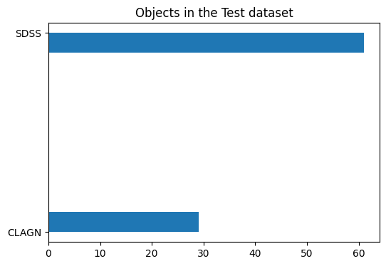
3.1 Train test split

We use sklearn’s train test split to randomly split the data into training and testing datasets. Because thre are uneven numbers of each type (many more SDSS than CLAGN), we want to make sure to stratify evenly by type.

#divide the dataframe into features and labels for ML algorithms
labels = df_lc[["objectid", "label"]].drop_duplicates().set_index("objectid").label
df_lc = df_lc.drop(columns=["label"]).set_index(["objectid", "datetime"])

test_size = 0.25

#want a stratified split based on label
train_ix, test_ix = train_test_split(df_lc.index.levels[0], stratify = labels, shuffle = True, random_state = 43, test_size = test_size)

#X is defined to be the features
#y is defined to be the labels
X_train = df_lc.loc[train_ix]
y_train = labels.loc[train_ix]
X_test = df_lc.loc[test_ix]
y_test = labels.loc[test_ix]

#plot to show how many of each type of object in the test dataset
plt.figure(figsize=(6,4))
plt.title("Objects in the Test dataset")
h = plt.hist(y_test, histtype='stepfilled', orientation='horizontal')

4. Run sktime algorithms on the light curves

We choose to use sktime algorithms beacuse it is a library of many algorithms specifically tailored to time series datasets. It is based on the sklearn library so syntax is familiar to many users.

Types of classifiers are listed here.

This notebook will first show you an example of a single algorithm classifier. Then it will show how to write a for loop over a bunch of classifiers while outputting some metrics of accuracy.

4.1 Check that the data types are ok for sktime

This test needs to pass in order for sktime to run

#ask sktime if it likes the data type of X_train
#if you change any of the functions or cells above this one, it is a good idea to
# look at the below output to make sure you haven't introduced any NaNs or unequal length series
check_is_mtype(X_train, mtype="pd-multiindex", scitype="Panel", return_metadata=True)

(True,
 None,
 {'is_univariate': False,
  'is_empty': False,
  'has_nans': np.False_,
  'n_features': 9,
  'feature_names': ['flux_W1',
   'flux_W2',
   'flux_panstarrs_g',
   'flux_panstarrs_i',
   'flux_panstarrs_r',
   'flux_panstarrs_y',
   'flux_panstarrs_z',
   'flux_zg',
   'flux_zr'],
  'dtypekind_dfip': [<DtypeKind.FLOAT: 2>,
   <DtypeKind.FLOAT: 2>,
   <DtypeKind.FLOAT: 2>,
   <DtypeKind.FLOAT: 2>,
   <DtypeKind.FLOAT: 2>,
   <DtypeKind.FLOAT: 2>,
   <DtypeKind.FLOAT: 2>,
   <DtypeKind.FLOAT: 2>,
   <DtypeKind.FLOAT: 2>],
  'feature_kind': [<DtypeKind.FLOAT: 2>,
   <DtypeKind.FLOAT: 2>,
   <DtypeKind.FLOAT: 2>,
   <DtypeKind.FLOAT: 2>,
   <DtypeKind.FLOAT: 2>,
   <DtypeKind.FLOAT: 2>,
   <DtypeKind.FLOAT: 2>,
   <DtypeKind.FLOAT: 2>,
   <DtypeKind.FLOAT: 2>],
  'n_instances': 267,
  'is_one_series': False,
  'is_equal_length': np.True_,
  'is_equally_spaced': True,
  'n_panels': 1,
  'is_one_panel': True,
  'mtype': 'pd-multiindex',
  'scitype': 'Panel'})

#show the list of all possible classifiers that work with multivariate data
#all_tags(estimator_types = 'classifier')
#classifiers = all_estimators("classifier", filter_tags={'capability:multivariate':True})
#classifiers

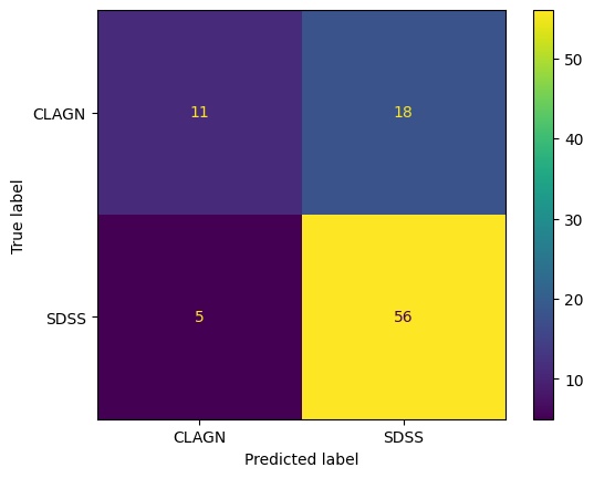
4.1 A single Classifier

%%time
#this cell takes 35s to run on a sample of 267 light curves

#setup the classifier
#n_jobs is the number of jobs to run in parallel. some environments have trouble with this.
#if you encounter an error such as 'BrokenProcessPool' while training or predicting, you may
#want to either set n_jobs = 1 or use a different compute environment.
clf = Arsenal(time_limit_in_minutes=1, n_jobs = -1)  # '-1' n_jobs means use all processors

#fit the classifier on the training dataset
clf.fit(X_train, y_train)

#make predictions on the test dataset using the trained model
y_pred = clf.predict(X_test)

print(f"Accuracy of Random Interval Classifier: {accuracy_score(y_test, y_pred)}\n", flush=True)

#plot a confusion matrix
cm = confusion_matrix(y_test, y_pred, labels=clf.classes_)
disp = ConfusionMatrixDisplay(confusion_matrix=cm,display_labels=clf.classes_)
disp.plot()

plt.show()

Accuracy of Random Interval Classifier: 0.7444444444444445

CPU times: user 2.37 s, sys: 931 ms, total: 3.3 s
Wall time: 1min 15s

4.2 Loop over a bunch of classifiers

Our method is to do a cursory check of a bunch of classifiers and then later drill down deeper on anything with good initial results. We choose to run a loop over ~10 classifiers that seem promising and check the accuracy scores for each one. Any classifier with a promising accuracy score could then be followed up with detailed hyperparameter tuning, or potentially with considering other classifiers in that same type.

#show the summary of the algorithms used and their accuracy score
#accscore_dict

#save statistics from these runs

# Serialize data into file:
#json.dump( accscore_dict, open( "output/accscore.json", 'w' ) )
#json.dump( completeness_dict, open( "output/completeness.json", 'w' ) )
#json.dump( homogeneity_dict, open( "output/homogeneity.json", 'w' ) )

# Read data from file:
#accscore_dict = json.load( open( "output/accscore.json") )

5.0 Create a candidate list

Lets assume we now have a classifier which can accurately differentiate CLAGN from SDSS QSOs based on their archival light curves. Next, we would like to use that classifier on our favorite unlabeled sample to identify CLAGN candidates. To do this, we need to:

• read in a dataframe of our new sample

• get that dataset in the same format as what was fed into the classifiers

• use your trained classifier to predict labels for the new sample

• retrace those objectids to an ra & dec

• write an observing proposal (ok, you have to do that one yourself)

#read in a dataframe of our new sample:
# we are going to cheat here and use the same file as we used for input to the above, but you should
# replace this with your favorite sample run through the light_curve_generator in this same repo.
path_to_sample = './data/small_CLAGN_SDSS_df_lc.parquet'
my_sample = pd.read_parquet(path_to_sample)

#get dataset in same format as what was run through sktime
#This is not exactly the same as re-running the whole notebook on a different sample,
#but it is pretty close.  We don't need to do all of the same cleaning because some of that
#was to appease sktime in training the algorithms.


#get rid of indices set in the light curve code and reset them as needed before sktime algorithms
my_sample = my_sample.reset_index()

# get rid of some of the bands that don't have enough data for all the sources
#CLAGN are generall fainter targets, and therefore mostly not found in datasets like TESS & K2
#make sure your sample has the same bands as were run to train the classifier
my_sample = my_sample[~my_sample["band"].isin(bands_to_drop)]

#drop rows which have Nans
my_sample.dropna(inplace = True, axis = 0)

#remove outliers
#make sure your sample has the same sigmaclip_value as was run to train the classifier
my_sample = sigmaclip_lightcurves(my_sample, sigmaclip_value, include_plot = False, verbose= False)

#remove objects without W1 fluxes
my_sample = remove_objects_without_band(my_sample, 'W1', verbose=False)

#remove incomplete data
#make sure your sample has the same threshold_too_few as were run to train the classifier
my_sample = remove_incomplete_data(my_sample, threshold_too_few, verbose = False)

#drop missing bands
my_sample = missingdata_drop_bands(my_sample, bands_to_keep, verbose = False)

#make arrays have uniform length and spacing
#make sure your sample has the same final_feq_interpol as was run to train the classifier
df_interpol = uniform_length_spacing(my_sample, final_freq_interpol, include_plot = False )
my_sample = df_interpol.explode(["time", "flux","err"], ignore_index=True)
my_sample = my_sample.astype({col: "float" for col in ["time", "flux", "err"]})

#reformat the data to have columns be the different flux bands
my_sample = reformat_df(my_sample)

#normalize
my_sample = local_normalization_max(my_sample, norm_column = "flux_W1")

#make datetime column
my_sample['datetime'] = mjd_to_datetime(my_sample)

#set index expected by sktime
my_sample = my_sample.set_index(["objectid", "label", "datetime"])

#drop the uncertainty and time columns
my_sample.drop(columns = ['err_panstarrs_g',	'err_panstarrs_i',	'err_panstarrs_r',	'err_panstarrs_y',
                          'err_panstarrs_z',	'err_W1',	'err_W2',	'err_zg',	'err_zr','time'], inplace = True)

 #make X
X_mysample  = my_sample.droplevel('label')

#what does this look like to make sure we are on track
X_mysample

		flux_W1	flux_W2	flux_panstarrs_g	flux_panstarrs_i	flux_panstarrs_r	flux_panstarrs_y	flux_panstarrs_z	flux_zg	flux_zr
objectid	datetime
1	2009-06-03 06:37:08.765742	1.000000	0.927367	0.140308	0.331437	0.267991	0.461279	0.464892	0.116756	0.286475
	2009-08-02 06:37:08.765742	1.000000	0.927367	0.140308	0.331437	0.267991	0.461279	0.464892	0.116756	0.286475
	2009-10-01 06:37:08.765742	1.000000	0.927367	0.140308	0.331437	0.267991	0.461279	0.464892	0.116756	0.286475
	2009-11-30 06:37:08.765742	1.000000	0.927367	0.140308	0.331437	0.267991	0.461279	0.464892	0.116756	0.286475
	2010-01-29 06:37:08.765742	1.000000	0.927367	0.140308	0.331437	0.267991	0.461279	0.464892	0.116756	0.286475
...	...	...	...	...	...	...	...	...	...	...
458	2022-07-25 06:37:08.765742	0.787245	0.568910	0.118627	0.414211	0.219828	0.393996	0.406282	0.125963	0.283218
	2022-09-23 06:37:08.765742	0.787245	0.568910	0.118627	0.414211	0.219828	0.393996	0.406282	0.125963	0.311635
	2022-11-22 06:37:08.765742	0.787245	0.568910	0.118627	0.414211	0.219828	0.393996	0.406282	0.135551	0.311296
	2023-01-21 06:37:08.765742	0.787245	0.568910	0.118627	0.414211	0.219828	0.393996	0.406282	0.139684	0.305088
	2023-03-22 06:37:08.765742	0.787245	0.568910	0.118627	0.414211	0.219828	0.393996	0.406282	0.127343	0.265804

30345 rows × 9 columns

#use the trained sktime algorithm to make predictions on the test dataset
y_mysample = clf.predict(X_mysample)

#access the sample_table made in the light curve generator notebook
#has information about the sample including ra & dec
savename_sample = './data/small_CLAGN_SDSS_sample.ecsv'
gdd.download_file_from_google_drive(file_id='1pSEKVP4LbrdWQK9ws3CaI90m3Z_2fazL',
                                    dest_path=savename_sample,
                                    unzip=True)
sample_table = Table.read(savename_sample, format='ascii.ecsv')

Downloading 1pSEKVP4LbrdWQK9ws3CaI90m3Z_2fazL into ./data/small_CLAGN_SDSS_sample.ecsv... 

Done.
Unzipping...

/home/runner/work/fornax-demo-notebooks/fornax-demo-notebooks/.tox/py311-buildhtml/lib/python3.11/site-packages/google_drive_downloader/google_drive_downloader.py:78: UserWarning: Ignoring `unzip` since "1pSEKVP4LbrdWQK9ws3CaI90m3Z_2fazL" does not look like a valid zip file
  warnings.warn('Ignoring `unzip` since "{}" does not look like a valid zip file'.format(file_id))

#associate these predicted CLAGN with RA & Dec

#need to first associate objectid with each of y_mysample
#make a new df with a column = objectid which
#includes all the unique objectids.
test = X_mysample.reset_index()
mysample_CLAGN = pd.DataFrame(test.objectid.unique(), columns = ['objectid'])
mysample_CLAGN["predicted_label"] = pd.Series(y_mysample)

#if I am only interested in the CLAGN, could drop anything with label = SDSS
querystring = 'predicted_label == "SDSS"'
mysample_CLAGN = mysample_CLAGN.drop(mysample_CLAGN.query(querystring ).index)

#then will need to merge candidate_CLAGN with sample_table along objectid
sample_table_df = sample_table.to_pandas()
candidate_CLAGN = pd.merge(mysample_CLAGN, sample_table_df, on = "objectid", how = "inner")

#show the CLAGN candidates ra & dec
candidate_CLAGN

	objectid	predicted_label	coord.ra	coord.dec	label
0	1	CLAGN	29.990000	0.553010	LaMassa 15
1	2	CLAGN	5.796083	0.588203	Green 22
2	3	CLAGN	36.483625	0.507417	MacLeod 16
3	5	CLAGN	150.584042	45.157583	MacLeod 16
4	6	CLAGN	155.468083	46.754333	MacLeod 16
...	...	...	...	...	...
97	204	CLAGN	171.400690	54.382555	SDSS
98	282	CLAGN	161.163170	38.759552	SDSS
99	314	CLAGN	259.412720	32.704313	SDSS
100	380	CLAGN	188.156210	66.414533	SDSS
101	415	CLAGN	200.730970	8.161559	SDSS

102 rows × 5 columns

Conclusions

Depending on your comfort level with the accuracy of the classifier you have trained, you could now write an observing proposal to confirm those targets prediced to be CLAGN based on their multiwavelength light curves.

References:

• “sktime: A Unified Interface for Machine Learning with Time Series” Markus Löning, Tony Bagnall, Sajaysurya Ganesh, George Oastler, Jason Lines, ViktorKaz, …, Aadesh Deshmukh (2020). sktime/sktime. Zenodo. http://doi.org/10.5281/zenodo.3749000

• “Scikit-learn: Machine Learning in Python”, Pedregosa et al., JMLR 12, pp. 2825-2830, 2011.

• “pandas-dev/pandas: Pandas” The pandas development team, 2020. Zenodo. https://doi.org/10.5281/zenodo.3509134

• This work made use of Astropy a community-developed core Python package and an ecosystem of tools and resources for astronomy (astropy:2013, astropy:2018, astropy:2022).