Cross-Match ZTF and Pan-STARRS using LSDB

Learning Goals

By the end of this tutorial, you will:

• understand how to cross-match cloud-based catalogs using lsdb.

• understand how to parallelize lsdb cross-matches using dask.

• have a feeling for when dask parallelization can be helpful.

• have a rough idea of the maximum number of objects that can be cross matched on each Fornax Science Console server type.

Introduction

In the era of increasingly large astronomical survey missions like TESS, Gaia, ZTF, Pan-STARRS, Roman, and Rubin, catalog operations are becoming less and less practical to complete on a personal computer. Operations such as source cross-matching can require many GB of memory and take many hours to complete using a single CPU. Recognizing these looming obstacles, many catalogs are becoming accessible to cloud computing platforms like the Fornax Science Console, and increasingly high-performance tools are being developed that leverage cloud computing resources to simplify and speed up catalog operations.

LSDB is a useful package for performing large cross-matches between HATS catalogs. It can leverage the Dask library to work with larger-than-memory data sets and distribute computation tasks across multiple cores. Users perform large cross-matches without ever having to download a file.

In this tutorial, we will use lsdb with dask to perform a cross-match between ZTF and Pan-STARRS HATS catalogs to benchmark the performance. These HATS catalogs are stored on AWS S3 cloud storage. An application might be to collect time-series photometry for 10,000 or more stars in the Kepler field from ZTF and Pan-STARRS. With this in mind, we will begin by cross-matching 10,000 sources from ZTF with the Pan-STARRS mean-object catalog. The user can choose to scale up to a larger number of rows to test the performance. The CSV file provided with this notebook contains the runtime results of tests run on various Fornax Science Console server types for comparison.

As of August 2025, the Fornax Science Console server types were:

• “Small” - 4 GB RAM, 2 CPU

• “Medium” - 16 GB RAM, 4 CPU

• “Large” - 64 GB RAM, 16 CPU

• “XLarge” - 512 GB RAM, 128 CPU

For generality, we will refer to the server type by the number of CPUs. For each server and each number of cross-match rows, we want to know the performance with (1) default dask configuration, (2) minimal dask - 1 worker, (3) bigger dask - as many workers as we can use, and (4) auto-scaling dask.

Note that in this notebook, only one configuration (combination of CPU count, number of cross-match rows, and dask configuration) is run at a time. It must be reconfigured and rerun to benchmark each configuration.

Runtime

As of August 2025, as written (10,000 rows with the “default” dask settings), this notebook takes about 45 seconds to run on the “small” Fornax Science Console server type (4 GB RAM and 2 CPUs). Users can modify the configuration for larger cross-matches, which will take more time. E.g., cross-matching 10 million rows on the “large” server type (64 GB RAM and 16 CPUs) can take ~5 minutes.

Imports

We require the following packages:

• os solely for the cpu_count function,

• datetime for measuring the crossmatch time,

• pandas to write and read the CSV of benchmarks

• matplotlib to plot the benchmarks,

• astropy for coordinates and units,

• lsdb to read the catalogs and perform the cross-match, and

• dask for parallelization.

# Uncomment the next line to install dependencies if needed.
# %pip install -r requirements_ztf_ps1_crossmatch.txt

from os import cpu_count
from datetime import datetime

import pandas as pd
import matplotlib.pyplot as plt
from astropy.coordinates import SkyCoord
from astropy import units as u

import lsdb
from lsdb.core.search import ConeSearch
from dask.distributed import Client, LocalCluster

1. Preconfiguring the Run

First choose the number of rows we want to cross-match and our dask environment. For tips on using dask with lsdb, see lsdb’s Dask Cluster Tips.

# The left table will have about this many rows. The cross-matched product will have slightly fewer.
# Set Nrows = -1 to cross-match the entire catalog. The full catalog cross-match is
# recommended ONLY on XLarge instance with at least 32 workers.
Nrows = 10_000

# dask_workers can be:
# - "default" (uses the default scheduler which runs all tasks in the main process)
# - an integer, which uses a fixed number of workers
# - "scale" to use an adaptive, auto-scaling cluster.
dask_workers = "default"

# The code in this cell is automatic setup based on the configuration in the previous cell, so it can be left alone.

# We must pass a radius to lsdb. Here is the mapping between radius and desired number of rows for ZTF.
# The values in this dictionary were determined experimentally, by
# incrementing/decrementing the radius until the desired number of
# catalog rows was returned.
radius = { # Nrows: radius_arcseconds
           10_000:     331,
          100_000:    1047,
        1_000_000:    3318,
       10_000_000:  11_180,
      100_000_000:  33_743,
    1_000_000_000: 102_000,
}

# Set up dask cluster
if dask_workers == "scale":
    cluster = LocalCluster()
    cluster.adapt(minimum_cores=1, maximum_cores=cpu_count())
    client = Client(cluster)
elif isinstance(dask_workers, int):
    client = Client(
        # Number of Dask workers - Python processes to run
        n_workers=dask_workers,
        # Limits number of Python threads per worker
        threads_per_worker=1,
        # Memory limit per worker
        memory_limit=None,
    )
elif dask_workers == "default":
    # Either using default configuration or configuring Dask
    # using the built-in DaskHub
    pass
else:
    raise ValueError("`dask_workers` must be one of 'default', 'scale' or an int.")

# The performance may depend on the number of CPUs available, so we'll track that as well.
num_cpus = cpu_count()

2. Read in catalogs and downselect ZTF to Nrows

# Define sky area. Here we're using the Kepler field.
c = SkyCoord('19:22:40  +44:30:00', unit=(u.hourangle, u.deg))
cone_ra, cone_dec = c.ra.value, c.dec.value

if Nrows > 0:
    radius_arcsec = radius[Nrows]
    search_filter = ConeSearch(cone_ra, cone_dec, radius_arcsec)
else:
    # Full cross-match
    # ONLY ON XLARGE ENVIRONMENT USING AT LEAST 32 CPUS
    search_filter = None

# Read ZTF DR23
ztf_path = "s3://ipac-irsa-ztf/contributed/dr23/objects/hats"
ztf_piece = lsdb.open_catalog(
    ztf_path,
    columns=["oid", "ra", "dec"],
    search_filter=search_filter
)

# Read Pan-STARRS DR2
ps1_path = "s3://stpubdata/panstarrs/ps1/public/hats/otmo"
ps1_margin = "s3://stpubdata/panstarrs/ps1/public/hats/otmo_10arcs"
ps1 = lsdb.open_catalog(
    ps1_path,
    margin_cache=ps1_margin,
    columns=["objName","objID","raMean","decMean"],
)

3. Initialize the crossmatch and compute, measuring the time elapsed.

# Setting up the cross-match actually takes very little time
ztf_x_ps1 = ztf_piece.crossmatch(ps1, radius_arcsec=1, n_neighbors=1, suffixes=("_ztf", "_ps1"))
ztf_x_ps1

lsdb Catalog ZTF_DR23_Objects_x_otmo:

	oid_ztf	ra_ztf	dec_ztf	objName_ps1	objID_ps1	raMean_ps1	decMean_ps1	_dist_arcsec
npartitions=16
Order: 6, Pixel: 15104	int64[pyarrow]	double[pyarrow]	double[pyarrow]	string[pyarrow]	int64[pyarrow]	double[pyarrow]	double[pyarrow]	double[pyarrow]
Order: 6, Pixel: 15105	...	...	...	...	...	...	...	...
...	...	...	...	...	...	...	...	...
Order: 6, Pixel: 15118	...	...	...	...	...	...	...	...
Order: 6, Pixel: 15119	...	...	...	...	...	...	...	...

8 out of 8 available columns in the catalog have been loaded lazily, meaning no data has been read, only the catalog schema

# Executing the cross-match does take time
t0 = datetime.now()
xmatch = ztf_x_ps1.compute()
t1 = datetime.now() - t0

print("Time Elapsed:", t1)

Time Elapsed: 0:00:13.237194

# Check the length of the resulting table
rows_out = len(xmatch)
print(f"Number of rows out: {rows_out:,d}")

Number of rows out: 8,593

# Close the Dask cluster/client when finished
if dask_workers != "default":
    if dask_workers == "scale":
        cluster.close()
    client.close()

4. Record and plot benchmarks

Write the recorded benchmark to an output file, then make plots to analyze the benchmarks.

try:
    # read in file if it exists
    benchmarks = pd.read_csv("output/xmatch_benchmarks.csv", index_col=["Ncpus", "Nrows", "Nworkers"])
except FileNotFoundError:
    # otherwise create an empty DataFrame
    multi_index = pd.MultiIndex(levels=[[], [], []], codes=[[], [], []], names=["Ncpus", "Nrows", "Nworkers"])
    benchmarks = pd.DataFrame(index=multi_index, columns=["time", "Nrows_out", "updated"])

# assign values
benchmarks.loc[
    (num_cpus, Nrows, dask_workers),
    ["time", "Nrows_out", "updated"]
    ] = t1.total_seconds(), int(rows_out), datetime.now().strftime("%Y-%m-%d %H:%M:%S")

benchmarks = benchmarks.sort_index()
# benchmarks.to_csv("output/xmatch_benchmarks.csv") # Uncomment this to write the new benchmarks to file
benchmarks

			time	Nrows_out	updated
Ncpus	Nrows	Nworkers
2	10000	1	48.879788	8593.0	2025-08-05 18:13:57
		2	30.538154	8593.0	2025-08-05 18:15:26
...	...	...	...	...	...
128	1000000000	default	1611.382256	874362668.0	2025-08-11 22:16:12
	7500000000	default	14539.090000	NaN	2025-08-12 21:37:39

125 rows × 3 columns

benchmarks = pd.read_csv("output/xmatch_benchmarks.csv", index_col=["Ncpus", "Nrows", "Nworkers"])

nworkers = [1, 2, 4, 8, 16, 32, 64, 128, 256, "default", "scale"]

def plot_by_nworkers(num_cpus, ax):
    # Plot execution time vs. number of dask workers for each scale job
    b = benchmarks.loc[num_cpus]

    for n in b.index.levels[0]:
        try:
            # get the relevant benchmarks
            b_N = b.xs(n, level="Nrows").reset_index()
        except KeyError:
            pass

        # convert Nworkers to categorical with desired order
        b_N["Nworkers"] = pd.Categorical(b_N["Nworkers"],
                                            categories=[str(x) for x in nworkers],
                                            ordered=True)
        b_N = b_N.sort_values("Nworkers")

        # only plot if there is more than 1 data point
        if len(b_N) > 1:
            ax.plot("Nworkers", "time", marker="s", linestyle="-", data=b_N, label=f"{n} rows")

    ax.set(yscale="log", xlabel="Nworkers", ylabel="Execution Time (s)",
           title=f"{num_cpus} CPUs")
    ax.legend()


fig, axs = plt.subplots(1, 4, figsize=(16, 4))
cpu_counts = benchmarks.index.get_level_values("Ncpus").drop_duplicates().sort_values()
for i, ncpu in enumerate(cpu_counts):
    plot_by_nworkers(ncpu, axs[i])
fig.tight_layout()

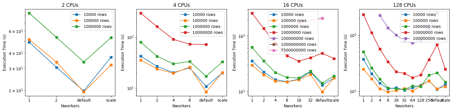
These plots show how the cross-match execution time depends on the number of workers used. Broadly, increasing the number of workers up to the number of available CPUs improves the performance. The exception is for smaller cross-matches ($\le$ 1 million rows) spread across many ($\ge$ 16) CPUs, when the overhead of managing many workers is significant compared to the cross-match time. Increasing the number of workers past the number of CPUs results in somewhat worse performance. Interestingly, the agnostic approach—not manually specifying any dask parameters, but instead letting lsdb use the default dask behavior—results in the best performance for smaller cross-matches. This indicates that the lsdb cross-match functions are well-optimized and well-configured for use with dask without much user oversight, at least on cross-matches with $\le$ 1 million rows.

For the largest jobs (Nrows $\ge$ 10 million), the default dask configuration performs worse than fixing the number of dask_workers to be the number of available CPUs. Interestingly, on the XLarge server with 128 CPUs, the 64-worker run performed the best on the large cross-matches. For larger cross-matches, we recommend manually setting the number of workers to be $\frac{1}{2} N_\mathrm{CPU} \leq N_\mathrm{workers} \leq N_\mathrm{CPU}$.

Given the amount of time it takes to perform the largest cross-matches (Nrows $\ge$ 1 billion), these were run only on the XLarge server using the default dask configuration. The full cross-match of over 7 billion rows took just over 4 hours.

These graphs also illustrate the approximate maximum number of rows that can be cross matched with a given amount of RAM and CPU. Trying to cross-match more rows or use worker configurations that aren’t shown in the plots can lead to one of the following behaviors:

Small (4GB RAM, 2 CPU)

When attempting Nrows $\ge$ 10 million, the cross-match exhibits long compute times, seeming never to finish.

Medium (16GB RAM, 4 CPU)

When attempting Nrows $\ge$ 100 million, the cross-match exhibits long compute times, seeming never to finish.

Large (64GB RAM, 16 CPU)

When attempting Nrows = 100 million with anything but 16 or ‘default’ values for dask_workers, the cross-match exhibits long compute times, seeming never to finish. When attempting Nrows $\ge$ 1 billion, the cross-match exhibits long compute times, seeming never to finish.

XLarge (512GB RAM, 128 CPU)

The XLarge environment was able to complete all attempted cross-matches, except that setting dask_workers='scale' resulted in the dead worker behavior documented below.

Autoscaling on any environment

When using dask_workers='scale' and scaling up the number of rows to cross-match, eventually you will see logging output from the dask cluster indicating that workers have died and are being respawn. This behavior repeats, and the cross-match never finishes (after being allowed to run for, e.g., an hour when it is expected to finish in 5 minutes).

5. Summary

The Fornax Science Console is capable of hosting cross-matches between large catalogs using the lsdb package. lsdb leverages dask to efficiently plan cross-match jobs using multiple workers, which results in large performance gains, especially as jobs scale up to millions or tens of millions of catalog rows.

Recommendations

• For small cross-matches (1 million rows or less) it is acceptable and often optimal to use lsdb’s default dask settings to parallelize jobs. In other words, for these jobs you don’t need to configure or even import dask at all to leverage its parallelization power.

• For large cross-matches (millions of rows or more), we recommend running in an environment with at least tens of CPUs, and setting the number of dask workers to at least half the number of available CPUs, and up to the number of CPUs. E.g., 128 CPUs with 64 dask workers.

• Cross-matches of 10 million rows or less can, at the time of writing, be completed on the Small Fornax Console using the default dask configuration. However, given the performance, we recommend the following use scaling:

  • Nrows $\le 10^6$: Small

  • $10^6 <$ Nrows $< 10^7$: Medium

  • $10^7 <$ Nrows $< 10^8$: Large

  • Nrows $> 10^8$: XLarge

In this tutorial we have cross-matched sections of catalogs in a particular region of sky, where most of the stars likely fall in the same or neighboring sky cells. It would be useful in the future to try this using generic samples of stars from across the entire sky. How different is performance when the catalog rows come from many sky cells instead of just a few? We have also generated the cross-match using compute, which loads the full result into memory, but lsdb supports larger-than-memory cross-matches by writing them directly to disk using to_hats. It would also be illustrative to run these benchmarks, and benchmarking a full cross-match between ZTF and Pan-STARRS, by writing the result to disk.

Other Science Cases

The example science case used here is an investigation to collect time-series photometry from sources in and around the Kepler field. The time series associated with the ZTF and Pan-STARRS sources might be used to supplement the Kepler light curves, extend their time baseline, examine how stellar light curves change in different photometric filters, and more. But lsdb enables other science cases with other catalogs as well. Some examples might be to

• combine photometric spectral energy distributions (SEDs) of distant galaxies with their spectra to build a training set for machine learning to predict photometric redshifts,

• combine Gaia’s exquisite astrometry with your favorite star survey to obtain 6D kinematic solutions for your sample stars,

• combine stellar spectroscopic catalogs with light curve rotation period measurements to estimate stellar ages using gyrochronology.

About this Notebook

• Authors: Zach Claytor (Astronomical Data Scientist at Space Telescope Science Institute) and the Fornax team

• Contact: For help with this notebook, please open a topic in the Fornax Community Forum “Support” category.

References

• This work uses astropy.

• This work uses lsdb.