Learning Goals
By the end of this tutorial, you will:
Work with multi-band lightcurve data
Learn high dimensional manifold of light curves with UMAPs and SOMs
Visualize and compare different samples on reduced dimension projections/grids
Introduction
Active Galactic Nuclei (AGNs), some of the most powerful sources in the universe, emit a broad range of electromagnetic radiation, from radio waves to gamma rays. Consequently, there is a wide variety of AGN labels depending on the identification/selection scheme and the presence or absence of certain emissions (e.g., Radio loud/quiet, Quasars, Blazars, Seiferts, Changing looks). According to the unified model, this zoo of labels we see depend on a limited number of parameters, namely the viewing angle, the accretion rate, presence or lack of jets, and perhaps the properties of the host/environment (e.g., Padovani et al. 2017). Here, we collect archival photometry and labels from the literature to compare how some of these different labels/selection schemes compare.
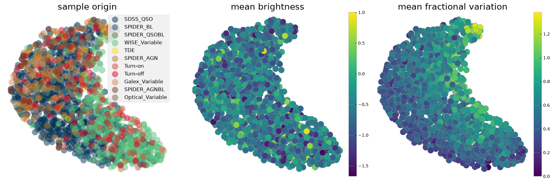
We use manifold learning and dimensionality reduction to learn the distribution of AGN lightcurves observed with different facilities. We mostly focus on UMAP (Uniform Manifold Approximation and Projection, McInnes 2020) but also show SOM (Self organizing Map, Kohonen 1990) examples. The reduced 2D projections from these two unsupervised ML techniques reveal similarities and overlaps of different selection techniques. Coloring the projections with various statistical physical properties (e.g., mean brightness, fractional lightcurve variation) is informative of correlations of the selections technique with physics such as AGN variability. Using different parts of the EM in training (or in building the initial higher dimensional manifold) demonstrates how much information if any is in that part of the data for each labeling scheme, for example whether with ZTF optical light curves alone, we can identify sources with variability in WISE near IR bands. These techniques also have a potential for identifying targets of a specific class or characteristic for future follow up observations.
Runtime
As of 2024 September, this notebook takes about 3 minutes to run to completion on Fornax using a server with 16 GB RAM and 4 CPU.
Imports
Here are the libraries used in this network. They are also mostly mentioned in the requirements in case you don’t have them installed.
sysandosto handle file names, paths, and directoriesnumpyandpandasto handle array functionsmatplotlibpyplotandcmfor plotting dataastropy.io.fitsfor accessing FITS filesastropy.table.Tablefor creating tidy tables of the dataAGNzoo_functionsfor reading in and prepreocessing of lightcurve dataumapandminisomfor manifold learning, dimensionality reduction, and visualization
This cell will install them if needed:
# Uncomment the next line to install dependencies if needed.
# %pip install -r requirements_ML_AGNzoo.txt
import sys
import astropy.units as u
from astropy.table import Table
import matplotlib.pyplot as plt
from matplotlib.colors import LinearSegmentedColormap
import matplotlib.gridspec as gridspec
from mpl_toolkits.axes_grid1 import make_axes_locatable
import numpy as np
import pandas as pd
sys.path.append('code_src/')
from AGNzoo_functions import (unify_lc, unify_lc_gp, stat_bands, autopct_format, combine_bands,
normalize_clipmax_objects, shuffle_datalabel, dtw_distance,
stretch_small_values_arctan, translate_bitwise_sum_to_labels, update_bitsums)
from collections import Counter, defaultdict
import umap
from minisom import MiniSom
import logging
# Get the root logger
logger = logging.getLogger()
logger.setLevel(logging.WARNING)
plt.style.use('bmh')
colors = [
"#3F51B5", # Ultramarine Blue
"#003153", # Prussian Blue
"#0047AB", # Cobalt Blue
"#40826D", # Viridian Green
"#50C878", # Emerald Green
"#FFEA00", # Chrome Yellow
"#CC7722", # Yellow Ochre
"#E34234", # Vermilion
"#E30022", # Cadmium Red
"#D68A59", # Raw Sienna
"#8A360F", # Burnt Sienna
"#826644", # Raw Umber
]
custom_cmap = LinearSegmentedColormap.from_list("custom_theme", colors[1:])1. Loading data
Here we load a parquet file of light curves generated using the light_curve_collector notebook in this same GitHub repo. With that light_curve_collector notebook, you can build your favorite sample from different sources in the literature and grab the data from archives of interest. This sample contains both spatial coordinates and categorical labels for each AGN. The labels are generated by a bitwise addition of a set of binary indicators. Each binary indicator corresponds to the AGN’s membership in various categories, such as being an SDSS_QSO or a WISE_Variable. For example, an AGN that is both an SDSS_QSO, a WISE_Variable, and also shows ‘Turn_on’ characteristics, would have a label calculated by combining these specific binary indicators using bitwise addition.
%%bash

# To download the data file containing the light curves from Googledrive
gdown 1gb2vWn0V2unstElGTTrHIIWIftHbXJvz -O ./data/df_lc_020724.parquet.gzip
Downloading...
From (original): https://drive.google.com/uc?id=1gb2vWn0V2unstElGTTrHIIWIftHbXJvz
From (redirected): https://drive.google.com/uc?id=1gb2vWn0V2unstElGTTrHIIWIftHbXJvz&confirm=t&uuid=cc7ddbc4-5d87-492e-8b80-03386d6c6f36
To: /home/runner/work/fornax-demo-notebooks/fornax-demo-notebooks/light_curves/data/df_lc_020724.parquet.gzip
0%| | 0.00/243M [00:00<?, ?B/s] 0%| | 524k/243M [00:00<00:50, 4.83MB/s] 1%|▏ | 3.15M/243M [00:00<00:14, 16.1MB/s] 5%|▌ | 13.1M/243M [00:00<00:04, 49.6MB/s] 9%|▉ | 21.5M/243M [00:00<00:03, 57.9MB/s] 13%|█▎ | 32.5M/243M [00:00<00:02, 75.0MB/s] 18%|█▊ | 44.6M/243M [00:00<00:02, 87.7MB/s] 22%|██▏ | 53.5M/243M [00:00<00:02, 81.9MB/s] 27%|██▋ | 65.5M/243M [00:00<00:01, 92.3MB/s] 31%|███ | 75.0M/243M [00:00<00:01, 91.8MB/s] 36%|███▌ | 86.5M/243M [00:01<00:01, 97.9MB/s] 42%|████▏ | 101M/243M [00:01<00:01, 112MB/s] 49%|████▉ | 120M/243M [00:01<00:00, 134MB/s] 58%|█████▊ | 141M/243M [00:01<00:00, 154MB/s] 66%|██████▌ | 160M/243M [00:01<00:00, 168MB/s] 73%|███████▎ | 178M/243M [00:01<00:00, 141MB/s] 80%|███████▉ | 194M/243M [00:01<00:00, 146MB/s] 87%|████████▋ | 212M/243M [00:01<00:00, 156MB/s] 97%|█████████▋| 236M/243M [00:01<00:00, 177MB/s]100%|██████████| 243M/243M [00:02<00:00, 120MB/s]
df_lc = pd.read_parquet('data/df_lc_020724.parquet.gzip')

# remove 64 for SPIDER only as its too large compared to the rest of the labels
df_lc = df_lc[df_lc.index.get_level_values('label') != '64']
# remove all bitwise sums that had 64 in them
df_lc = update_bitsums(df_lc)df_lc1.1 What is in this sample
To effectively undertake machine learning (ML) in addressing a specific question, it’s imperative to have a clear understanding of the data we’ll be utilizing. This understanding aids in selecting the appropriate ML approach and, critically, allows for informed and necessary data preprocessing. For example whether a normalization is needed, and what band to choose for normalization.
objid = df_lc.index.get_level_values('objectid')[:].unique()
seen = Counter()

for (objectid, label), singleobj in df_lc.groupby(level=["objectid", "label"]):
    bitwise_sum = int(label)
    active_labels = translate_bitwise_sum_to_labels(bitwise_sum)
    seen.update(active_labels)
# changing order of labels in dictionary only for text to be readable on the plot
key_order = ('SDSS_QSO', 'SPIDER_AGN', 'SPIDER_BL', 'SPIDER_QSOBL', 'SPIDER_AGNBL',
             'WISE_Variable', 'Optical_Variable', 'Galex_Variable', 'Turn-on', 'Turn-off', 'TDE')
new_queue = {}
for k in key_order:
    new_queue[k] = seen[k]

plt.figure(figsize=(8, 8))
plt.title(r'Sample consists of:', size=15)
h = plt.pie(new_queue.values(), labels=new_queue.keys(), autopct=autopct_format(new_queue.values()),
            textprops={'fontsize': 15}, startangle=30, labeldistance=1.1,
            wedgeprops={'linewidth': 3, 'edgecolor': 'white'}, colors=colors)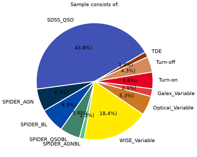
In this particular example, the largest subsamples of AGNs, all with a criteria on redshift (z<1), are from the optical spectra by the SDSS quasar sample DR16Q, the value added SDSS spectra from SPIDERS, and a subset of AGNs selected in MIR WISE bands based on their variability (csv in data folder credit RChary). We also include some smaller samples from the literature to see where they sit compared to the rest of the population and if they are localized on the 2D projection. These include the Changing Look AGNs from the literature (e.g., LaMassa et al. 2015, Lyu et al. 2022, Hon et al. 2022), a sample which showed variability in Galex UV images (Wasleske et al. 2022), a sample of variable sources identified in optical Palomar observations (Baldassare et al. 2020), and the optically variable AGNs in the COSMOS field from a three year program on the VLT(De Cicco et al. 2019). We also include 30 Tidal Disruption Event coordinates identified from ZTF light curves Hammerstein et al. (2022).
seen = Counter()
seen = df_lc.reset_index().groupby('band').objectid.nunique().to_dict()

plt.figure(figsize=(20, 4))
plt.title(r'Number of lightcurves in each waveband in this sample:', size=20)
h = plt.bar(seen.keys(), seen.values())
plt.ylabel(r'#', size=20)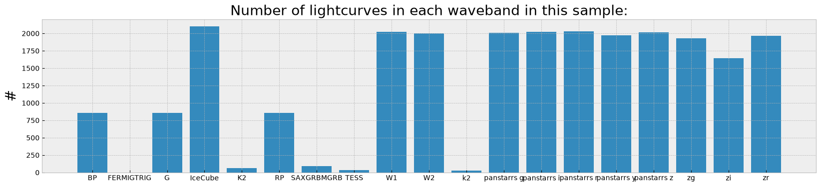
The histogram shows the number of lightcurves which ended up in the multi-index data frame from each of the archive calls in different wavebands/filters.
cadence = dict((el, []) for el in seen.keys())
timerange = dict((el, []) for el in seen.keys())

for (_, band), times in df_lc.reset_index().groupby(["objectid", "band"]).time:
    cadence[band].append(len(times))
    if times.max() - times.min() > 0:
        timerange[band].append(np.round(times.max() - times.min(), 1))

plt.figure(figsize=(20, 4))
plt.title(r'Time range and cadence covered in each in each waveband averaged over this sample:')
for el in cadence.keys():
    plt.scatter(np.mean(timerange[el]), np.mean(cadence[el]), label=el, s=len(timerange[el]))
    plt.errorbar(np.mean(timerange[el]), np.mean(cadence[el]),
                 xerr=np.std(timerange[el]), yerr=np.std(cadence[el]), alpha=0.2)
    plt.annotate(el, (np.mean(timerange[el]), np.mean(cadence[el])+2), size=12, rotation=40)
plt.ylabel(r'Average number of visits', size=20)
plt.xlabel(r'Average baseline (days)', size=20)
plt.xlim([0, 4000])
plt.yscale('log')
/home/runner/work/fornax-demo-notebooks/fornax-demo-notebooks/.tox/py313-buildhtml/lib/python3.13/site-packages/numpy/_core/fromnumeric.py:3860: RuntimeWarning: Mean of empty slice.
return _methods._mean(a, axis=axis, dtype=dtype,
/home/runner/work/fornax-demo-notebooks/fornax-demo-notebooks/.tox/py313-buildhtml/lib/python3.13/site-packages/numpy/_core/_methods.py:144: RuntimeWarning: invalid value encountered in scalar divide
ret = ret.dtype.type(ret / rcount)
/home/runner/work/fornax-demo-notebooks/fornax-demo-notebooks/.tox/py313-buildhtml/lib/python3.13/site-packages/numpy/_core/_methods.py:222: RuntimeWarning: Degrees of freedom <= 0 for slice
ret = _var(a, axis=axis, dtype=dtype, out=out, ddof=ddof,
/home/runner/work/fornax-demo-notebooks/fornax-demo-notebooks/.tox/py313-buildhtml/lib/python3.13/site-packages/numpy/_core/_methods.py:180: RuntimeWarning: invalid value encountered in divide
arrmean = um.true_divide(arrmean, div, out=arrmean,
/home/runner/work/fornax-demo-notebooks/fornax-demo-notebooks/.tox/py313-buildhtml/lib/python3.13/site-packages/numpy/_core/_methods.py:214: RuntimeWarning: invalid value encountered in scalar divide
ret = ret.dtype.type(ret / rcount)
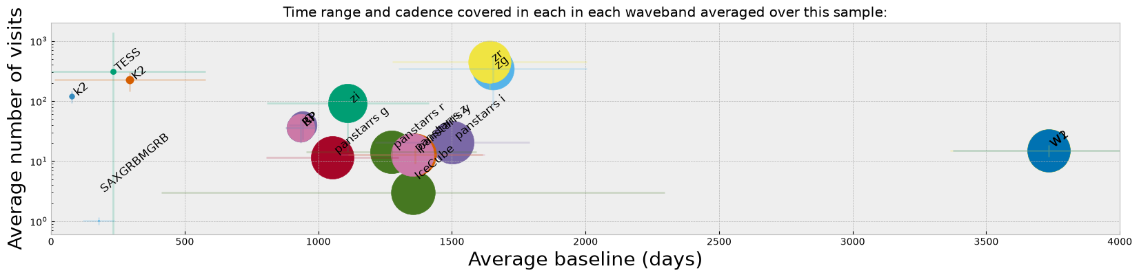
While from the histogram plot we see which bands have the highest number of observed lightcurves, what might matter more in finding/selecting variability or changing look in lightcurves is the cadence and the average baseline of observations. For instance, Panstarrs has a large number of lightcurve detections in our sample, but from the figure above we see that the average number of visits and the baseline for those observations are considerably less than ZTF. WISE also shows the longest baseline of observations which is suitable to finding longer term variability in objects.
2. Preprocess data for ML (ZTF bands)
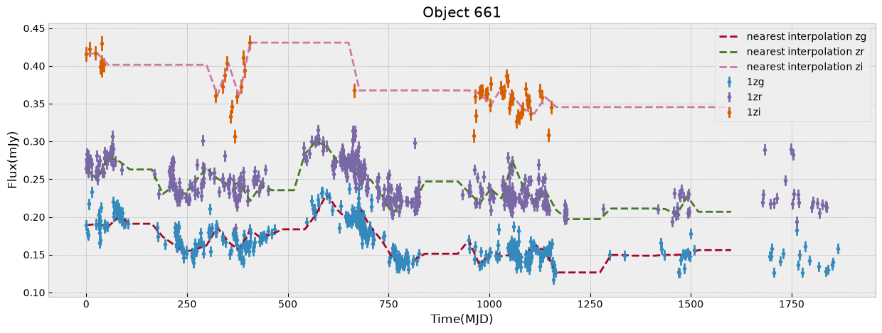
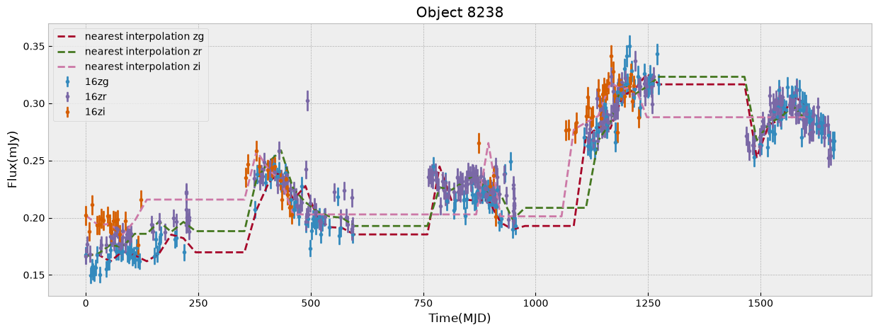
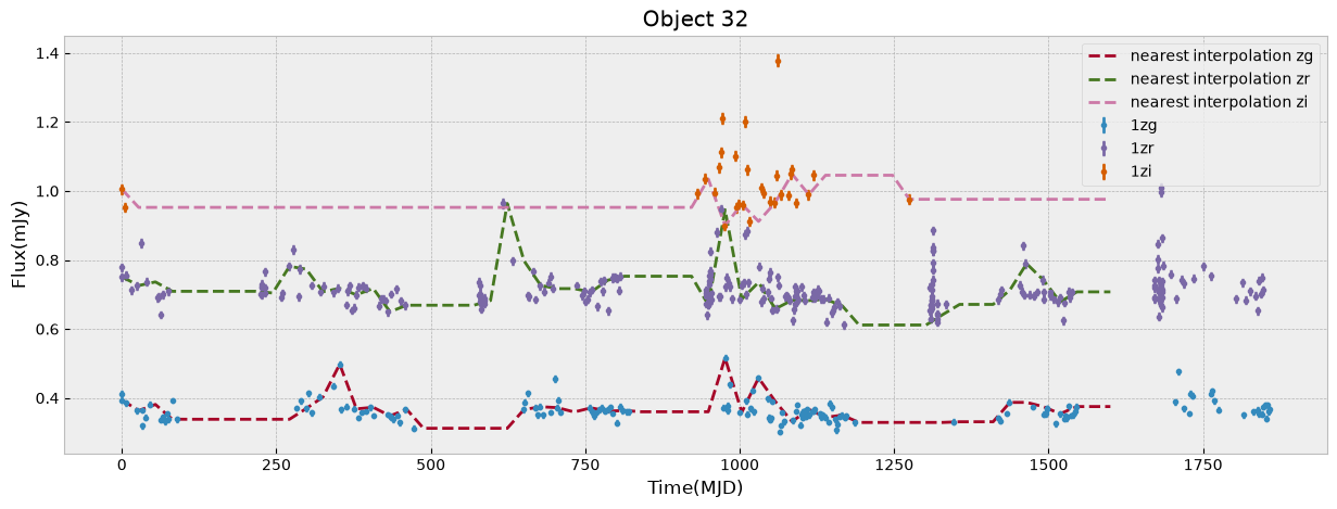
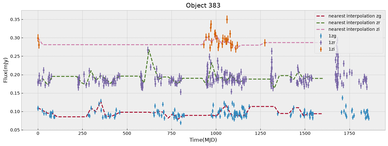
We first look at this sample only in ZTF bands which have the largest number of visits. We start by unifying the time grid of the light curves so oobjects with different start time or number of observations can be compared. We do this by interpolation to a new grid. The choice of the grid resolution and baseline is strictly dependent on the input data, in this case ZTF, to preserve as much as possible all the information from the observations. The unify_lc, or unify_lc_gp functions do the unification of the lightcurve arrays. For details please see the codes. The time arrays are chosen based on the average duration of observations, with ZTF and WISE covering 1600, 4000 days respectively. We note that we disregard the time of observation of each source, by subtracting the initial time from the array and bringing all lightcurves to the same footing. This has to be taken into account if it influences the science of interest. We then interoplate the time arrays with linear or Gaussian Process regression (unift_lc/ unify_lc_gp respectively). We also remove from the sample objects with less than 5 datapoints in their light curve. We measure basic statistics and combine the tree observed ZTF bands into one longer array as input to dimensionailty reduction after deciding on normalization. We also do a shuffling of the sample to be sure that the separations of different classes by ML are not simply due to the order they are seen in training (in case it is not done by the ML routine itself).
bands_inlc = ['zg', 'zr', 'zi']

# nearest neighbor linear interpolation:
objects, dobjects, flabels, keeps = unify_lc(df_lc, bands_inlc, xres=60, numplots=5,
                                             low_limit_size=5)

# Gaussian process unification
# objects, dobjects, flabels, keeps = unify_lc_gp(df_lc, bands_inlc, xres=60, numplots=5,
#                                                 low_limit_size=5)

# keeps can be used as index of objects that are kept in "objects" from the initial "df_lc",
# in case information about some properties of sample (e.g., redshifts) is of interest
# this array of indecies would be helpful

# calculate some basic statistics with a sigmaclipping with width 5sigma
fvar, maxarray, meanarray = stat_bands(objects, dobjects, bands_inlc, sigmacl=5)

# combine different waveband into one array
dat_notnormal = combine_bands(objects, bands_inlc)

# Normalize the combinde array by maximum of brightness in a waveband after clipping outliers:
dat = normalize_clipmax_objects(dat_notnormal, maxarray, band=1)

# Normalize the combinde array by mean brightness in a waveband after clipping outliers:
datm = normalize_clipmax_objects(dat_notnormal, meanarray, band=1)

# shuffle data incase the ML routines are sensitive to order
data, fzr, p = shuffle_datalabel(dat, flabels)
fvar_arr, maximum_arr, average_arr = fvar[:, p], maxarray[:, p], meanarray[:, p]

# Initialize labc to hold indices of each unique label
labc = {}
for index, f in enumerate(fzr):
    lab = translate_bitwise_sum_to_labels(int(f))
    for label in lab:
        if label not in labc:
            # Initialize the list for this label if it's not already in labc
            labc[label] = []
        # Append the current index to the list of indices for this label
        labc[label].append(index)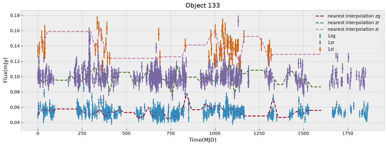
/home/runner/work/fornax-demo-notebooks/fornax-demo-notebooks/light_curves/code_src/AGNzoo_functions.py:290: RuntimeWarning: invalid value encountered in sqrt
  fvar = (np.sqrt(varf - deltaf)) / meanf
The combination of the tree bands into one longer arrays in order of increasing wavelength, can be seen as providing both the SED shape as well as variability in each from the light curve. Figure below demonstrates this as well as our normalization choice. We normalize the data in ZTF R band as it has a higher average numbe of visits compared to G and I band. We remove outliers before measuring the mean and max of the light curve and normalizing by it. This normalization can be skipped if one is mearly interested in comparing brightnesses of the data in this sample, but as dependence on flux is strong to look for variability and compare shapes of light curves a normalization helps.
r = np.random.randint(np.shape(dat)[1])

_, axs = plt.subplots(1, 3, figsize=(18, 4))
ztf_data = [dat_notnormal, dat, datm]
ylabels = [r'Flux ($\mu Jy$)', r'Normalized Flux (max r band)', r'Normalized Flux (mean r band)']
fig_contents = list(zip(axs, ztf_data, ylabels))

for i, l in enumerate(bands_inlc):
    s = int(np.shape(dat)[1]/len(bands_inlc))
    first = int(i*s)
    last = first+s
    for ax, ydata, ylabel in fig_contents:
        ax.plot(np.linspace(first, last, s), ydata[r, first:last], 'o', linestyle='--', label=l)
        ax.set_xlabel(r'Time_[w1, w2, w3]', size=15)
        ax.set_ylabel(ylabel, size=15)
_ = axs[0].legend(loc=2)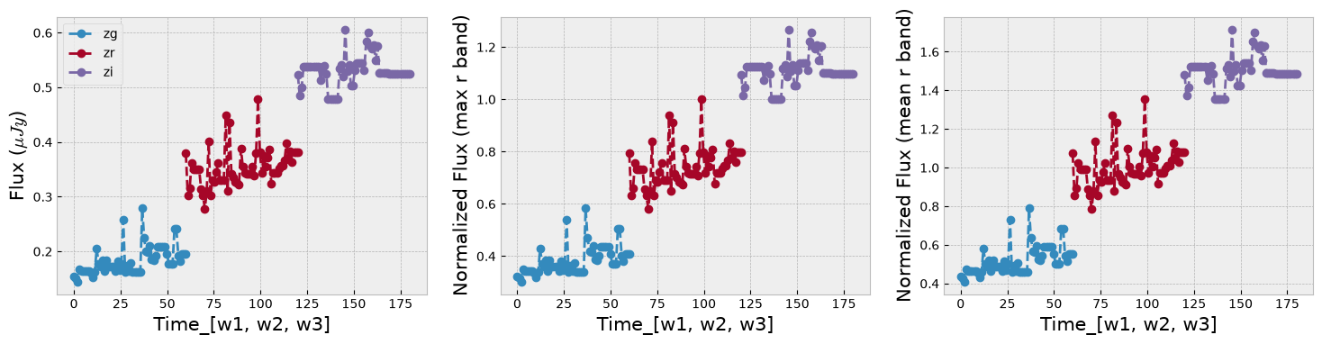
3. Learn the Manifold
Now we can train a UMAP with the processed data vectors above. Different choices for the number of neighbors, minimum distance and metric can be made and a parameter space can be explored. We show here our preferred combination given this data. We choose manhattan distance (also called the L1 distance) as it is optimal for the kind of grid we interpolated on, for instance we want the distance to not change if there are observations missing. Another metric appropriate for our purpose in time domain analysis is Dynamic Time Warping (DTW), which is insensitive to a shift in time. This is helpful as we interpolate the observations onto a grid starting from time 0 and when discussing variability we care less about when it happens and more about whether and how strong it happened. As the measurement of the DTW distance takes longer compared to the other metrics we show examples here with manhattan and only show one example exploring the parameter space including a DTW metric in the last cell of this notebook.
plt.figure(figsize=(18, 6))
markersize=200
mapper = umap.UMAP(n_neighbors=50, min_dist=0.9, metric='manhattan', random_state=20).fit(data)


ax1 = plt.subplot(1, 3, 2)
ax1.set_title(r'mean brightness', size=20)
cf = ax1.scatter(mapper.embedding_[:, 0], mapper.embedding_[:, 1], s=markersize,
                 c=np.log10(np.nansum(meanarray, axis=0)), edgecolor='gray')
plt.axis('off')
divider = make_axes_locatable(ax1)
cax = divider.append_axes("right", size="5%", pad=0.05)
plt.colorbar(cf, cax=cax)


ax0 = plt.subplot(1, 3, 3)
ax0.set_title(r'mean fractional variation', size=20)
cf = ax0.scatter(mapper.embedding_[:, 0], mapper.embedding_[:, 1], s=markersize,
                 c=stretch_small_values_arctan(np.nansum(fvar_arr, axis=0), factor=3),
                 edgecolor='gray')
plt.axis('off')
divider = make_axes_locatable(ax0)
cax = divider.append_axes("right", size="5%", pad=0.05)
plt.colorbar(cf, cax=cax)

ax2 = plt.subplot(1, 3, 1)
ax2.set_title('sample origin', size=20)
counts = 1
for label, indices in labc.items():
    cf = ax2.scatter(mapper.embedding_[indices, 0], mapper.embedding_[indices, 1], s=markersize,
                     c=colors[counts], alpha=0.5, edgecolor='gray', label=label)
    counts += 1
plt.legend(fontsize=12)
#plt.colorbar(cf)
plt.axis('off')

plt.tight_layout()
#plt.savefig('umap-ztf.png')
/home/runner/work/fornax-demo-notebooks/fornax-demo-notebooks/.tox/py313-buildhtml/lib/python3.13/site-packages/umap/umap_.py:1952: UserWarning: n_jobs value 1 overridden to 1 by setting random_state. Use no seed for parallelism.
warn(
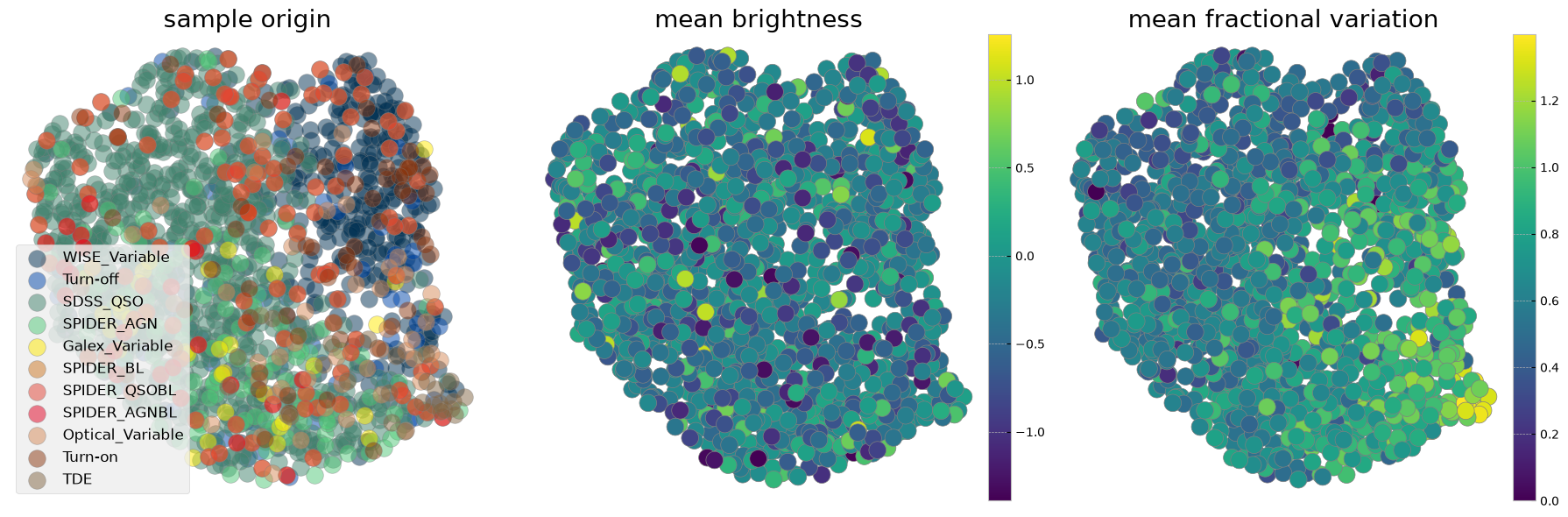
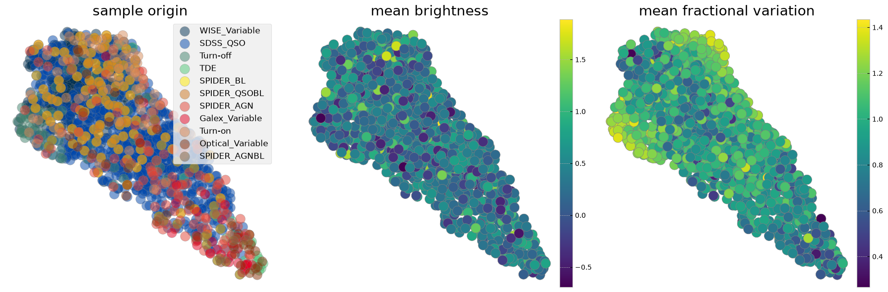
The left panel is colorcoded by the origin of the sample. The middle panel shows the sum of mean brightnesses in three bands (arbitrary unit) demonstrating that after normalization we see no correlation with brightness. The panel on the right is color coded by a statistical measure of variability (i.e. the fractional variation see here). As with the plotting above it is not easy to see all the data points and correlations in the next two cells measure probability of belonging to each original sample as well as the mean statistical property on an interpolated grid on this reduced 2D projected surface.
# Define a grid
grid_resolution = 15# Number of cells in the grid
x_min, x_max = mapper.embedding_[:, 0].min(), mapper.embedding_[:, 0].max()
y_min, y_max = mapper.embedding_[:, 1].min(), mapper.embedding_[:, 1].max()
x_grid = np.linspace(x_min, x_max, grid_resolution)
y_grid = np.linspace(y_min, y_max, grid_resolution)
x_centers, y_centers = np.meshgrid(x_grid, y_grid)
# Calculate mean property in each grid cell
mean_property1, mean_property2 = np.zeros_like(x_centers), np.zeros_like(x_centers)
propmean=stretch_small_values_arctan(np.nansum(meanarray, axis=0), factor=2)
propfvar=stretch_small_values_arctan(np.nansum(fvar_arr, axis=0), factor=2)
for i in range(grid_resolution - 1):
for j in range(grid_resolution - 1):
mask = (
(mapper.embedding_[:, 0] >= x_grid[i]) &
(mapper.embedding_[:, 0] < x_grid[i + 1]) &
(mapper.embedding_[:, 1] >= y_grid[j]) &
(mapper.embedding_[:, 1] < y_grid[j + 1])
)
if np.sum(mask) > 0:
mean_property1[j, i] = np.mean(propmean[mask])
mean_property2[j, i] = np.mean(propfvar[mask])
plt.figure(figsize=(12, 4))
plt.subplot(1, 2, 1)
plt.title('mean brightness')
cf = plt.contourf(x_centers, y_centers, mean_property1, cmap='viridis', alpha=0.9)
plt.axis('off')
divider = make_axes_locatable(plt.gca())
cax = divider.append_axes("right", size="5%", pad=0.05)
plt.colorbar(cf, cax=cax)
plt.subplot(1, 2, 2)
plt.title('mean fractional variation')
cf = plt.contourf(x_centers, y_centers, mean_property2, cmap='viridis', alpha=0.9)
plt.axis('off')
divider = make_axes_locatable(plt.gca())
cax = divider.append_axes("right", size="5%", pad=0.05)
plt.colorbar(cf, cax=cax)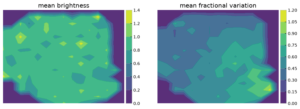
3.1 Sample comparison on the UMAP
# Calculate 2D histogram
hist, x_edges, y_edges = np.histogram2d(mapper.embedding_[:, 0], mapper.embedding_[:, 1], bins=12)
plt.figure(figsize=(15, 12))
i=1
ax0 = plt.subplot(4, 4, 12)
for label, indices in sorted(labc.items()):
hist_per_cluster, _, _ = np.histogram2d(mapper.embedding_[indices, 0],
mapper.embedding_[indices, 1],
bins=(x_edges, y_edges))
prob = hist_per_cluster / hist
plt.subplot(4, 4, i)
plt.title(label)
plt.contourf(x_edges[:-1], y_edges[:-1], prob.T, levels=20, alpha=0.8, cmap=custom_cmap)
plt.colorbar()
plt.axis('off')
cf = ax0.scatter(mapper.embedding_[indices, 0], mapper.embedding_[indices, 1], s=80,
alpha=0.5, edgecolor='gray', label=label, c=colors[i-1])
i += 1
ax0.legend(loc=4, fontsize=7)
ax0.axis('off')
plt.tight_layout()/tmp/ipykernel_3628/3793995111.py:10: RuntimeWarning: invalid value encountered in divide
prob = hist_per_cluster / hist
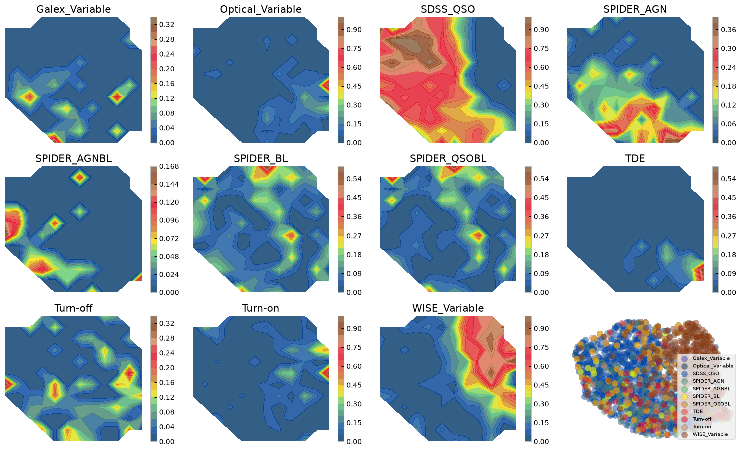
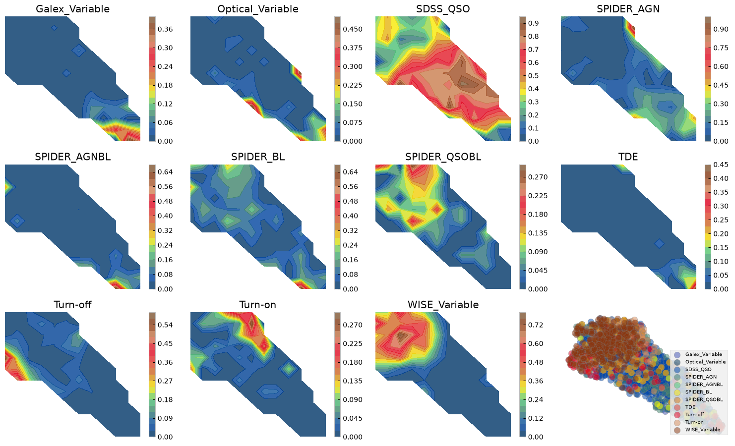
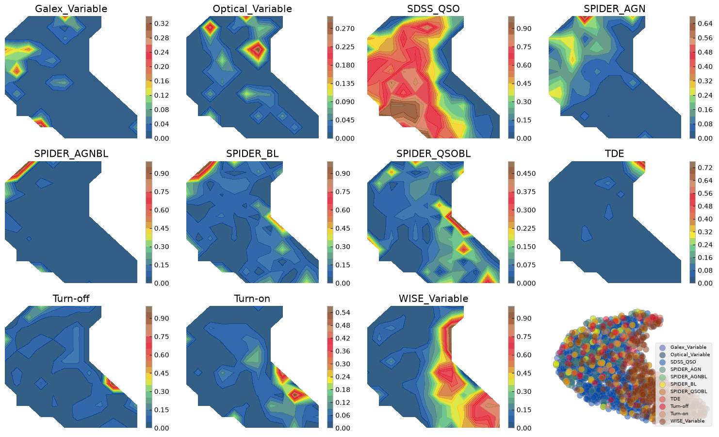
Figure above shows how with ZTF light curves alone we can separate some of these AGN samples, where they have overlaps. We can do a similar exercise with other dimensionality reduction techniques. Below we show two SOMs one with normalized and another with no normalization. The advantage of Umaps to SOMs is that in practice you may change the parameters to separate classes of vastly different data points, as distance is preserved on a umap. On a SOM however only topology of higher dimensions is preserved and not distance hence, the change on the 2d grid does not need to be smooth and from one cell to next there might be larg jumps. On the other hand, an advantage of the SOM is that by definition it has a grid and no need for a posterior interpolation (as we did above) is needed to map more data or to measure probabilities, etc.
3.2 Reduced dimensions on a SOM grid
# Initialization and training
msz0, msz1 = 15, 15
som = MiniSom(msz0, msz1, data.shape[1], sigma=1.5, learning_rate=.5,
neighborhood_function='gaussian', random_seed=0, topology='rectangular')
som.pca_weights_init(data)
som.train(data, 100000, verbose=False) # random traininglaborder = ['SDSS_QSO', 'SPIDER_AGN', 'SPIDER_BL', 'SPIDER_QSOBL', 'SPIDER_AGNBL',
'WISE_Variable', 'Optical_Variable', 'Galex_Variable', 'Turn-on', 'Turn-off', 'TDE']
# Create grid to hold mean fvar per SOM node
mean_fvar_map = np.full((msz0, msz1), np.nan)
# Create helper to accumulate fvar values in each cell
cell_fvar = defaultdict(list)
# First, map each data point to its BMU and store its fvar
propfvar=stretch_small_values_arctan(np.nansum(fvar_arr, axis=0), factor=2)
for i in range(len(data)):
bmu = som.winner(data[i]) # returns (x, y)
fvar_value = fvar_arr[i] if np.ndim(fvar_arr) == 1 else np.mean(propfvar[i])
cell_fvar[bmu].append(fvar_value)
# Now compute mean per cell
for (x, y), values in cell_fvar.items():
mean_fvar_map[x, y] = np.nanmean(values)
# apply stretching for visualization
heatmap = stretch_small_values_arctan(mean_fvar_map)
ncols = 4
nrows = int(np.ceil(len(laborder) / ncols))
fig, axs = plt.subplots(nrows, ncols, figsize=(3*ncols, 3*nrows))
axs = axs.flatten()
for i, label in enumerate(laborder):
ax = axs[i]
im = ax.imshow(heatmap.T, origin='lower', cmap='plasma')
if label in labc:
for idx in labc[label]:
x, y = som.winner(data[idx])
ax.plot(x, y, 'x', color='white', markersize=8, markeredgewidth=2)
ax.set_title(label)
ax.set_xticks([])
ax.set_yticks([])
# Hide the extra subplot if laborder < nrows * ncols
if len(laborder) < len(axs):
axs[len(laborder)].axis('off')
# Colorbar outside the plot grid
# Adjust position as needed (here it's to the right)
cbar_ax = fig.add_axes([0.99, 0.05, 0.02, 0.9]) # [left, bottom, width, height]
cbar = fig.colorbar(im, cax=cbar_ax)
cbar.set_label('Mean Fractional Variability')
plt.subplots_adjust(right=0.9) # Leave space for colorbar
plt.tight_layout()
plt.show()/tmp/ipykernel_3628/2599028209.py:53: UserWarning: This figure includes Axes that are not compatible with tight_layout, so results might be incorrect.
plt.tight_layout()
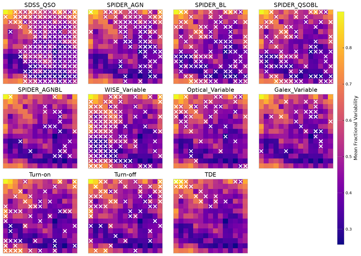
The above SOMs are colored by the mean fractional variation of the lightcurves in all bands (a measure of AGN variability). The crosses are different samples mapped to the trained SOM to see if they are distinguishable on a normalized lightcurve som.
# shuffle data in case the ML routines are sensitive to order
data, fzr, p = shuffle_datalabel(dat_notnormal, flabels)
fvar_arr, maximum_arr, average_arr = fvar[:, p], maxarray[:, p], meanarray[:, p]
# Initialize labc to hold indices of each unique label
labc = {}
for index, f in enumerate(fzr):
lab = translate_bitwise_sum_to_labels(int(f))
for label in lab:
if label not in labc:
# Initialize the list for this label if it's not already in labc
labc[label] = []
# Append the current index to the list of indices for this label
labc[label].append(index)
som = MiniSom(msz0, msz1, data.shape[1], sigma=1.5, learning_rate=.5,
neighborhood_function='gaussian', random_seed=0, topology='rectangular')
som.pca_weights_init(data)
som.train(data, 100000, verbose=False) # random training# Create grid to hold mean fvar per SOM node
mean_fvar_map = np.full((msz0, msz1), np.nan)
# Create helper to accumulate fvar values in each cell
cell_fvar = defaultdict(list)
# First, map each data point to its BMU and store its fvar
propfvar=stretch_small_values_arctan(np.nansum(fvar_arr, axis=0), factor=2)
for i in range(len(data)):
bmu = som.winner(data[i]) # returns (x, y)
fvar_value = fvar_arr[i] if np.ndim(fvar_arr) == 1 else np.mean(propfvar[i])
cell_fvar[bmu].append(fvar_value)
# Now compute mean per cell
for (x, y), values in cell_fvar.items():
mean_fvar_map[x, y] = np.nanmean(values)
# apply stretching for visualization
heatmap = stretch_small_values_arctan(mean_fvar_map)
ncols = 4
nrows = int(np.ceil(len(laborder) / ncols))
fig, axs = plt.subplots(nrows, ncols, figsize=(3*ncols, 3*nrows))
axs = axs.flatten()
for i, label in enumerate(laborder):
ax = axs[i]
im = ax.imshow(heatmap.T, origin='lower', cmap='plasma')
if label in labc:
for idx in labc[label]:
x, y = som.winner(data[idx])
ax.plot(x, y, 'x', color='white', markersize=8, markeredgewidth=2)
ax.set_title(label)
ax.set_xticks([])
ax.set_yticks([])
# Hide the extra subplot if laborder < nrows * ncols
if len(laborder) < len(axs):
axs[len(laborder)].axis('off')
# Colorbar outside the plot grid
# Adjust position as needed (here it's to the right)
cbar_ax = fig.add_axes([0.99, 0.05, 0.02, 0.9]) # [left, bottom, width, height]
cbar = fig.colorbar(im, cax=cbar_ax)
cbar.set_label('Mean Fractional Variability')
plt.subplots_adjust(right=0.9) # Leave space for colorbar
plt.tight_layout()
plt.show()/tmp/ipykernel_3628/1301010532.py:49: UserWarning: This figure includes Axes that are not compatible with tight_layout, so results might be incorrect.
plt.tight_layout()
labels = [None] * len(data)
for label in laborder:
if label in labc:
for idx in labc[label]:
labels[idx] = label
labels_map = defaultdict(Counter)
for x, label in zip(data, labels):
if label is not None:
w = som.winner(x)
labels_map[w][label] += 1
fig = plt.figure(figsize=(12, 12))
the_grid = gridspec.GridSpec(msz0, msz1, fig)
for position in labels_map.keys():
label_counts = labels_map[position]
total = sum(label_counts.values())
# Use consistent order from laborder
fracs = [label_counts.get(label, 0) / total for label in laborder]
ax = plt.subplot(the_grid[msz1 - 1 - position[1], position[0]], aspect=1)
patches, _ = ax.pie(fracs)
#ax.set_title(f"{position}", fontsize=6)
ax.axis('equal')
# Legend outside
plt.legend(patches, laborder, bbox_to_anchor=(1.05, 1), loc='upper left', fontsize=8)
plt.tight_layout()
plt.show()/tmp/ipykernel_3628/2695913503.py:31: UserWarning: Tight layout not applied. tight_layout cannot make Axes width small enough to accommodate all Axes decorations
plt.tight_layout()
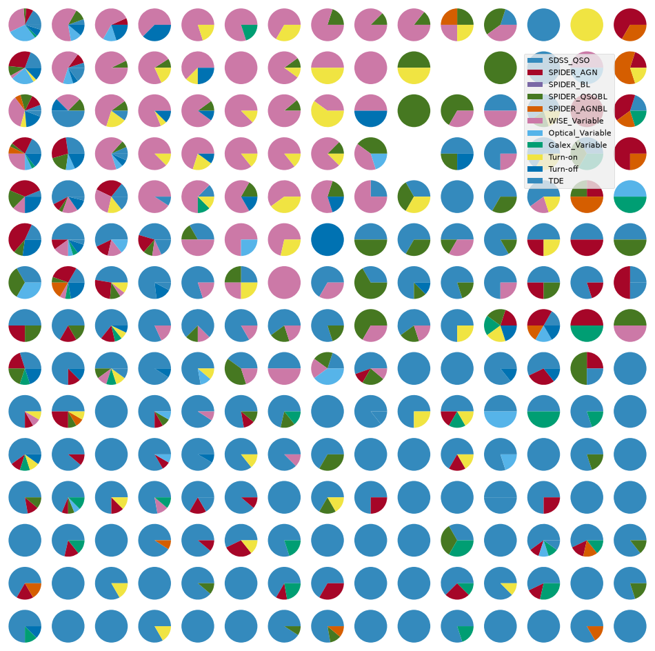
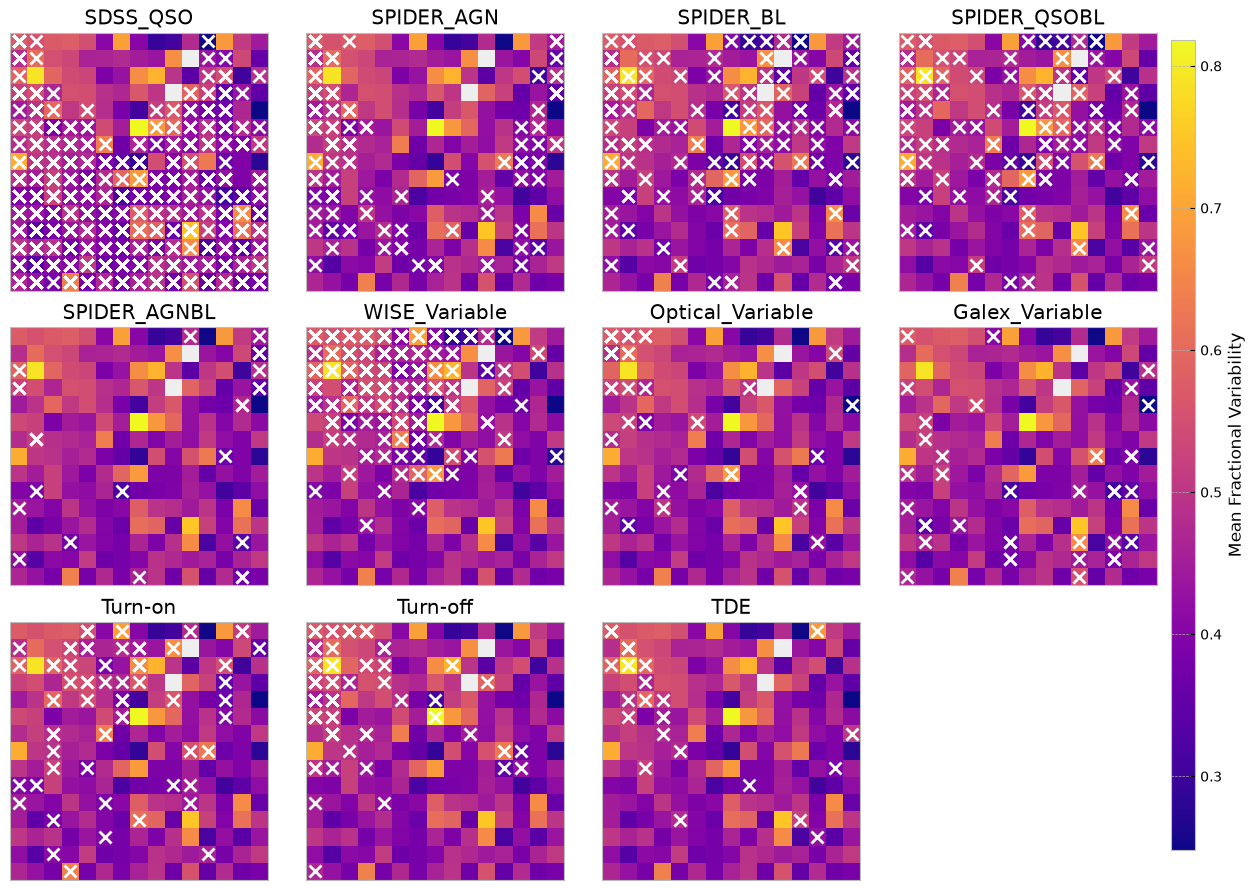
skipping the normalization of lightcurves, further separates turn on/off CLAGNs when looking at ZTF lightcurves only.
4. Repeating the above, this time with ZTF + WISE manifold
bands_inlc = ['zg', 'zr', 'zi', 'W1', 'W2']
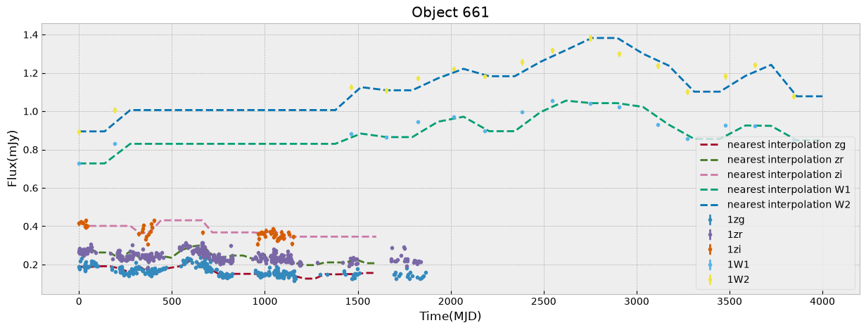
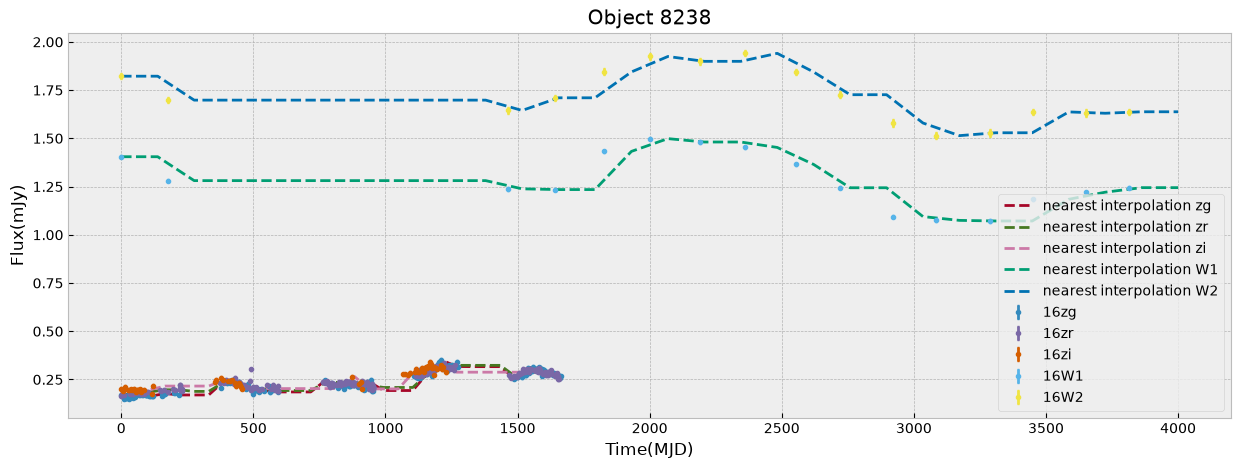
objects, dobjects, flabels, keeps = unify_lc(df_lc, bands_inlc, xres=30, numplots=3)
# calculate some basic statistics
fvar, maxarray, meanarray = stat_bands(objects, dobjects, bands_inlc)
dat_notnormal = combine_bands(objects, bands_inlc)
dat = normalize_clipmax_objects(dat_notnormal, maxarray, band=-1)
data, fzr, p = shuffle_datalabel(dat, flabels)
fvar_arr, maximum_arr, average_arr = fvar[:, p], maxarray[:, p], meanarray[:, p]
# Initialize labc to hold indices of each unique label
labc = {}
for index, f in enumerate(fzr):
lab = translate_bitwise_sum_to_labels(int(f))
for label in lab:
if label not in labc:
# Initialize the list for this label if it's not already in labc
labc[label] = []
# Append the current index to the list of indices for this label
labc[label].append(index)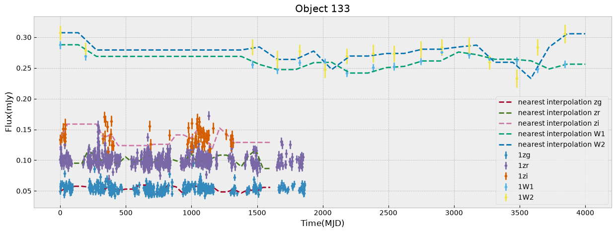
/home/runner/work/fornax-demo-notebooks/fornax-demo-notebooks/light_curves/code_src/AGNzoo_functions.py:290: RuntimeWarning: invalid value encountered in sqrt
fvar = (np.sqrt(varf - deltaf)) / meanf
plt.figure(figsize=(18, 6))
markersize=200
mapper = umap.UMAP(n_neighbors=50, min_dist=0.9, metric='manhattan', random_state=4).fit(data)
# using dtw distance takes a long time
# mapper = umap.UMAP(n_neighbors=50, min_dist=0.9, metric=dtw_distance, random_state=20).fit(data)
ax1 = plt.subplot(1, 3, 2)
ax1.set_title(r'mean brightness', size=20)
cf = ax1.scatter(mapper.embedding_[:, 0], mapper.embedding_[:, 1], s=markersize,
c=np.log10(np.nansum(meanarray, axis=0)), edgecolor='gray')
plt.axis('off')
divider = make_axes_locatable(ax1)
cax = divider.append_axes("right", size="5%", pad=0.05)
plt.colorbar(cf, cax=cax)
ax0 = plt.subplot(1, 3, 3)
ax0.set_title(r'mean fractional variation', size=20)
cf = ax0.scatter(mapper.embedding_[:, 0], mapper.embedding_[:, 1], s=markersize,
c=stretch_small_values_arctan(np.nansum(fvar_arr, axis=0), factor=3),
edgecolor='gray')
plt.axis('off')
divider = make_axes_locatable(ax0)
cax = divider.append_axes("right", size="5%", pad=0.05)
plt.colorbar(cf, cax=cax)
ax2 = plt.subplot(1, 3, 1)
ax2.set_title('sample origin', size=20)
counts = 1
for label, indices in labc.items():
cf = ax2.scatter(mapper.embedding_[indices, 0], mapper.embedding_[indices, 1], s=markersize,
c=colors[counts], alpha=0.5, edgecolor='gray', label=label)
counts += 1
plt.legend(fontsize=12)
#plt.colorbar(cf)
plt.axis('off')
plt.tight_layout()/home/runner/work/fornax-demo-notebooks/fornax-demo-notebooks/.tox/py313-buildhtml/lib/python3.13/site-packages/umap/umap_.py:1952: UserWarning: n_jobs value 1 overridden to 1 by setting random_state. Use no seed for parallelism.
warn(
# Calculate 2D histogram
hist, x_edges, y_edges = np.histogram2d(mapper.embedding_[:, 0], mapper.embedding_[:, 1], bins=12)
plt.figure(figsize=(15, 12))
i=1
ax0 = plt.subplot(4, 4, 12)
for label, indices in sorted(labc.items()):
hist_per_cluster, _, _ = np.histogram2d(mapper.embedding_[indices, 0],
mapper.embedding_[indices, 1],
bins=(x_edges, y_edges))
prob = hist_per_cluster / hist
plt.subplot(4, 4, i)
plt.title(label)
plt.contourf(x_edges[:-1], y_edges[:-1], prob.T, levels=20, alpha=0.8, cmap=custom_cmap)
plt.colorbar()
plt.axis('off')
cf = ax0.scatter(mapper.embedding_[indices, 0], mapper.embedding_[indices, 1], s=80,
alpha=0.5, edgecolor='gray', label=label, c=colors[i-1])
i += 1
ax0.legend(loc=4, fontsize=7)
ax0.axis('off')
plt.tight_layout()/tmp/ipykernel_3628/3793995111.py:10: RuntimeWarning: invalid value encountered in divide
prob = hist_per_cluster / hist
5. Wise bands alone
bands_inlcw = ['W1', 'W2']
objectsw, dobjectsw, flabelsw, keepsw = unify_lc(df_lc, bands_inlc, xres=30)
# calculate some basic statistics
fvarw, maxarrayw, meanarrayw = stat_bands(objectsw, dobjectsw, bands_inlcw)
dat_notnormalw = combine_bands(objects, bands_inlcw)
datw = normalize_clipmax_objects(dat_notnormalw, maxarrayw, band=-1)
dataw, fzrw, pw = shuffle_datalabel(datw, flabelsw)
fvar_arrw, maximum_arrw, average_arrw = fvarw[:, pw], maxarrayw[:, pw], meanarrayw[:, pw]
# Initialize labc to hold indices of each unique label
labcw = {}
for index, f in enumerate(fzrw):
lab = translate_bitwise_sum_to_labels(int(f))
for label in lab:
if label not in labcw:
# Initialize the list for this label if it's not already in labc
labcw[label] = []
# Append the current index to the list of indices for this label
labcw[label].append(index)/home/runner/work/fornax-demo-notebooks/fornax-demo-notebooks/light_curves/code_src/AGNzoo_functions.py:290: RuntimeWarning: invalid value encountered in sqrt
fvar = (np.sqrt(varf - deltaf)) / meanf
plt.figure(figsize=(18, 6))
markersize=200
mapp = umap.UMAP(n_neighbors=50, min_dist=0.9, metric='manhattan', random_state=20).fit(dataw)
ax1 = plt.subplot(1, 3, 2)
ax1.set_title(r'mean brightness', size=20)
cf = ax1.scatter(mapp.embedding_[:, 0], mapp.embedding_[:, 1], s=markersize,
c=np.log10(np.nansum(meanarrayw, axis=0)), edgecolor='gray')
plt.axis('off')
divider = make_axes_locatable(ax1)
cax = divider.append_axes("right", size="5%", pad=0.05)
plt.colorbar(cf, cax=cax)
ax0 = plt.subplot(1, 3, 3)
ax0.set_title(r'mean fractional variation', size=20)
cf = ax0.scatter(mapp.embedding_[:, 0], mapp.embedding_[:, 1], s=markersize,
c=stretch_small_values_arctan(np.nansum(fvar_arrw, axis=0), factor=3),
edgecolor='gray')
plt.axis('off')
divider = make_axes_locatable(ax0)
cax = divider.append_axes("right", size="5%", pad=0.05)
plt.colorbar(cf, cax=cax)
ax2 = plt.subplot(1, 3, 1)
ax2.set_title('sample origin', size=20)
counts = 1
for label, indices in labcw.items():
cf = ax2.scatter(mapp.embedding_[indices, 0], mapp.embedding_[indices, 1], s=markersize,
c=colors[counts], alpha=0.5, edgecolor='gray', label=label)
counts += 1
plt.legend(fontsize=12)
#plt.colorbar(cf)
plt.axis('off')
plt.tight_layout()/home/runner/work/fornax-demo-notebooks/fornax-demo-notebooks/.tox/py313-buildhtml/lib/python3.13/site-packages/umap/umap_.py:1952: UserWarning: n_jobs value 1 overridden to 1 by setting random_state. Use no seed for parallelism.
warn(
# Calculate 2D histogram
hist, x_edges, y_edges = np.histogram2d(mapp.embedding_[:, 0], mapp.embedding_[:, 1], bins=12)
plt.figure(figsize=(15, 12))
i=1
ax0 = plt.subplot(4, 4, 12)
for label, indices in sorted(labcw.items()):
hist_per_cluster, _, _ = np.histogram2d(mapp.embedding_[indices, 0],
mapp.embedding_[indices, 1],
bins=(x_edges, y_edges))
prob = hist_per_cluster / hist
plt.subplot(4, 4, i)
plt.title(label)
plt.contourf(x_edges[:-1], y_edges[:-1], prob.T, levels=20, alpha=0.8, cmap=custom_cmap)
plt.colorbar()
plt.axis('off')
cf = ax0.scatter(mapp.embedding_[indices, 0], mapp.embedding_[indices, 1], s=80,
alpha=0.5, edgecolor='gray', label=label, c=colors[i-1])
i += 1
ax0.legend(loc=4, fontsize=7)
ax0.axis('off')
plt.tight_layout()/tmp/ipykernel_3628/3463858432.py:10: RuntimeWarning: invalid value encountered in divide
prob = hist_per_cluster / hist
6. UMAP with different metrics/distances on ZTF+WISE
DTW takes a bit longer compared to other metrics, so it is commented out in the cell below.
plt.figure(figsize=(12, 10))
markersize=200
mapper = umap.UMAP(n_neighbors=50, min_dist=0.9, metric='euclidean', random_state=20).fit(data)
ax0 = plt.subplot(2, 2, 1)
ax0.set_title(r'Euclidean Distance, min_d=0.9, n_neighbors=50', size=12)
for label, indices in (labc.items()):
cf = ax0.scatter(mapper.embedding_[indices, 0], mapper.embedding_[indices, 1], s=80,
alpha=0.5, edgecolor='gray', label=label)
plt.axis('off')
mapper = umap.UMAP(n_neighbors=50, min_dist=0.9, metric='manhattan', random_state=20).fit(data)
ax0 = plt.subplot(2, 2, 2)
ax0.set_title(r'Manhattan Distance, min_d=0.9, n_neighbors=50', size=12)
for label, indices in (labc.items()):
cf = ax0.scatter(mapper.embedding_[indices, 0], mapper.embedding_[indices, 1], s=80,
alpha=0.5, edgecolor='gray', label=label)
plt.axis('off')
# This distance takes long
# mapperg = umap.UMAP(n_neighbors=50, min_dist=0.9, metric=dtw_distance, random_state=20).fit(data)
# ax2 = plt.subplot(2, 2, 3)
# ax2.set_title(r'DTW Distance, min_d=0.9, n_neighbors=50', size=12)
# for label, indices in (labc.items()):
# cf = ax2.scatter(mapper.embedding_[indices, 0], mapper.embedding_[indices, 1], s=80,
# alpha=0.5, edgecolor='gray', label=label)
# plt.axis('off')
mapper = umap.UMAP(n_neighbors=50, min_dist=0.1, metric='manhattan', random_state=20).fit(data)
ax0 = plt.subplot(2, 2, 4)
ax0.set_title(r'Manhattan Distance, min_d=0.1, n_neighbors=50', size=12)
for label, indices in (labc.items()):
cf = ax0.scatter(mapper.embedding_[indices, 0], mapper.embedding_[indices, 1], s=80,
alpha=0.5, edgecolor='gray', label=label)
plt.legend(fontsize=12)
plt.axis('off')/home/runner/work/fornax-demo-notebooks/fornax-demo-notebooks/.tox/py313-buildhtml/lib/python3.13/site-packages/umap/umap_.py:1952: UserWarning: n_jobs value 1 overridden to 1 by setting random_state. Use no seed for parallelism.
warn(
/home/runner/work/fornax-demo-notebooks/fornax-demo-notebooks/.tox/py313-buildhtml/lib/python3.13/site-packages/umap/umap_.py:1952: UserWarning: n_jobs value 1 overridden to 1 by setting random_state. Use no seed for parallelism.
  warn(
/home/runner/work/fornax-demo-notebooks/fornax-demo-notebooks/.tox/py313-buildhtml/lib/python3.13/site-packages/umap/umap_.py:1952: UserWarning: n_jobs value 1 overridden to 1 by setting random_state. Use no seed for parallelism.
  warn(
(np.float64(-3.8178215265274047),
 np.float64(10.599652791023255),
 np.float64(2.8609209060668945),
 np.float64(11.284222602844238))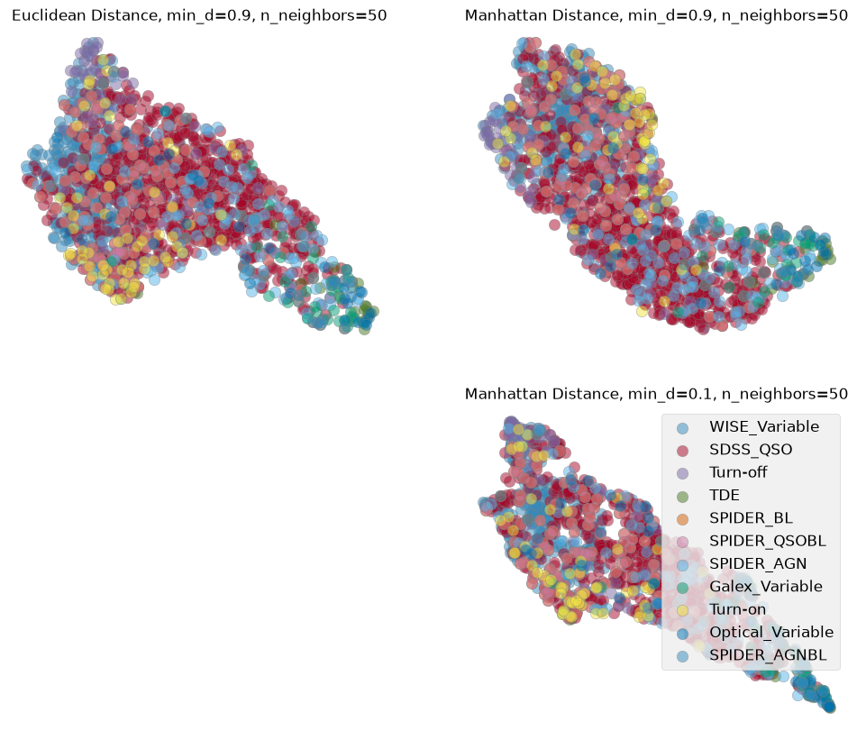
About this notebook
Authors: Shoubaneh Hemmati (IRSA Research Scientist) and the Fornax team
Contact: For help with this notebook, please open a topic in the Fornax Helpdesk.
Acknowledgements
Parts of this notebook will be presented in Hemmati et al. (in prep)
References
- Hammerstein, E., van Velzen, S., Gezari, S., Cenko, S. B., Yao, Y., Ward, C., Frederick, S., Villanueva, N., Somalwar, J. J., Graham, M. J., Kulkarni, S. R., Stern, D., Andreoni, I., Bellm, E. C., Dekany, R., Dhawan, S., Drake, A. J., Fremling, C., Gatkine, P., … Yan, L. (2022). The Final Season Reimagined: 30 Tidal Disruption Events from the ZTF-I Survey. The Astrophysical Journal, 942(1), 9. 10.3847/1538-4357/aca283